
UNSUPERVISED ARTIFICIAL NEURAL NETWORKS FOR
CLUSTERING OF DOCUMENT COLLECTIONS
Abdel-Badeeh M. Salem, Mostafa M. Syiam, and Ayad F. Ayad
Computer Science Department, Faculty of Computer & Information Sciences
Ain Shams University, Cairo, Egypt.
Keywords: Neural networks, Self-Organizing Map, Document Clustering.
Abstract: The Self-Organizing Map (SOM) has shown to be a stable neural network model for high- dimensional data
analy
sis. However, its applicability is limited by the fact that some knowledge about the data is required to
define the size of the network. In this paper the Growing Hierarchical SOM (GHSOM) is proposed. This
dynamically growing architecture evolves into a hierarchical structure of self–organizing maps according to
the characteristics of input data. Furthermore, each map is expanded until it represents the corresponding
subset of the data at specific level. We demonstrate the benefits of this novel model using a real world
example from the document-clustering domain. Comparison between both models (SOM & GHSOM) was
held to explain the difference and investigate the benefits of using GHSOM.
1 INTRODUCTION
The Self-Organizing Map (SOM) (Kohonen, 1982)
is an artificial neural network model that is well
suited for mapping high-dimensional data into a 2-
dimensional representation space. The training
process is based on weight vector adaptation with
respect to the input vectors. The SOM has shown to
be a highly effective tool for data visualization in a
broad spectrum of application domains (Kohonen,
1998) . Especially the utilization of the SOM for
information retrieval purposes in large free-form
document collections has gained wide interest in the
last few years (Lagus et Al., 1998) (Merkl, 1997)
(Rauber and Merkl, 2000). The general idea is to
display the contents of a document library by
representing similar documents in similar regions of
the map. One of the disadvantages of the SOM in
such an application area is its fixed size in terms of
the number of units and their particular arrangement,
which has to be defined prior to the start of the
training process. Without knowledge of the type and
the organization of the documents it is difficult to
get satisfying results without multiple training runs
using different parameter settings, which obviously
is extremely time consuming given the high-
dimensional data representation. Recently a number
of neural network models inspired by the training
process of the SOM and having adaptive
architectures were proposed (Fritzke, 1998). The
model being closest to the SOM is the so-called
Growing Grid (Fritzke, 1997), where a SOM-like
neural network grows dynamically during training.
The basic idea is to add rows or columns to the SOM
in those areas where the input vectors are not yet
represented sufficiently. More precisely, units are
added to those regions of the map where large
deviations between the input vectors and the weight
vector of the unit representing these input data are
observed. However, this method will produce very
large maps, which are difficult to survey and
therefore are not that suitable for large document
collections. Another possibility is to use a
hierarchical structure of independent SOMs
(Miikkulainen, 1995), where for every unit of a map
a SOM is added to the next layer. This means that on
the first layer of the Hierarchical Feature Map
(HFM) we obtain a rather rough representation of
the input space but with descending the hierarchy
the granularity increases. We believe that such an
approach is especially well suited for the
representation of the contents of a document
collection. The reason is that document collections
are inherently structured hierarchically with respect
to different subject matters. This is essentially the
way how conventional libraries are organized for
centuries. However, like with the original SOM, the
HFM uses a fixed architecture with a specified depth
383
M. Salem A., M. Syiam M. and F. Ayad A. (2004).
UNSUPERVISED ARTIFICIAL NEURAL NETWORKS FOR CLUSTERING OF DOCUMENT COLLECTIONS.
In Proceedings of the Sixth International Conference on Enterprise Information Systems, pages 383-392
DOI: 10.5220/0002595203830392
Copyright
c
SciTePress

of the hierarchy and predefined size of the various
SOMs on each layer. Again, we need profound
knowledge of the data in order to define a suitable
architecture. In order to combine the benefits of the
neural network models described above we
introduce a Growing Hierarchical SOM (GHSOM).
This model consists of a hierarchical architecture
where each layer is composed of independent SOMs
that adjust their size according to the requirements
of the input data. The remainder of the paper is
organized as follows. In section 2 we describe the
architecture and the training process of the GHSOM
The used data set and preprocessing steps are
demonstrated in section 3. The results of
experiments in document clustering with both SOM
and GHSOM are provided in section 4. Finally, we
present some conclusions in section 5.
.
2 GROWING HIERARCHICAL
SOM (GHSOM)
The key idea of the Growing Hierarchical Self-
Organizing Map (GHSOM) is to use a hierarchical
neural network structure composed of a number of
individual layers each of which consists of
independent self-organizing maps. In particular, the
neural network architecture starts with a single unit
SOM at layer 0. One SOM is used at layer 1of the
hierarchy. For every unit in this layer 1 map, a SOM
might be added to the next layer of the hierarchy.
This principal is repeated with the third and any
further layers of the GHSOM.
Since one of the shortcomings of the SOM usage is
its fixed network architecture in terms of the number
units and their arrangement, we rather rely on an
incrementally version of the SOM. This relieves us
from the burden of predefining the network’s size
which is now determined during the unsupervised
training process according to the peculiarities of the
input data space. Pragmatically speaking, the
GHSOM is intended to uncover the hierarchical
relationship between input data in a straightforward
fashion. More precisely, the similarities of the input
data are shown in increasingly finer levels of detail
along the hierarchy defined by the neural network
architecture. SOMs at higher layers give a coarse-
grained picture of the input data space whereas
SOMs of deeper layers provide fine-grained input
discrimination. The growth process of the neural
network is guided by the so-called quantization
error, which is a measure of the quality of the input
data representation.
The starting point for the growth process is the
overall deviation of the input data as measured with
the single unit SOM at layer 0. This unit is assigned
a weight vector m
0
, m
0
= [µ
01
, µ
02
, …, µ
0n
]
T
,
computed as the average of all input data. The
deviation of the input data, i.e. the mean
quantization error of this single unit, is computed as
given in expression (1) with d representing the
number of input data x. The mean quantization error
of a unit will be referred to as mqe in lower case
letters.
||||
1
00
xm
d
mqe −=
(1)
After the computation of mqe
0
, training of the
GHSOM starts with its first layer SOM. This first
layer map initially consists of a rather small number
of units, e.g. a grid of 2 x 2 units. Each of theses
units i is assigned an n-dimensional weight vector
m
i
, m
i =
[µ
i1
, µ
i2
,…, µ
in
]
T
, m
i Є R
n
, which is initialized
with random values. It’s important to note that
weight vectors have the same dimensionality as the
input patterns.
The learning process of SOMs may be described as a
competition among the units to represent the input
patterns. The unit with the weight vector being
closest to the presented input pattern in terms of
input space wins the competition. The weight vector
of the winner as well as units in the vicinity of the
winner are adapted in such a way as to resemble
more closely the input pattern (Salem et Al., 2003).
The degree of the adaptation is guided by means of a
learning rate parameter α, decreasing in time. The
number of units that are subject to adaptation also
decreases in time such that at the beginning of the
learning process a large number of units around the
winner are adapted, whereas towards the end only
the winner is adapted. These units are chosen by
means of a neighborhood function h
ci
, which is
based on the units’ distances to the winner as
measured in the 2-dimensional grid formed by the
neural network. In combining these principles of
SOM training, the learning rule may be written as
given in expression (2), where x represents the
current input pattern, and c refers to the winner at
iteration t
m
i
(t+1) = m
i
(t) + α(t) h
ci
(t) [x(t)- m
i
(t)]
In order to adapt the size of this first layer SOM, the
mean quantization error of the map is computed ever
after a fixed number λ of training iterations as given
in expression (3). In this formula, u refers to the
number of units i contained in the SOM m. In
analogy to expression (1), mqe
i
is computed as the
average distance between weight vector m
i
and the
input patterns mapped onto unit i. The mean
quantization error of a map will be referred to as
MQE in upper case letters.
ICEIS 2004 - ARTIFICIAL INTELLIGENCE AND DECISION SUPPORT SYSTEMS
384
The basic idea is that each layer of the GHSOM is
responsible for explaining some portion of the
deviation of the input data as present in its preceding
layer. This is done by adding units to the SOMs on
each layer until a suitable size of the map is reached.
More precisely, the SOMs on each layer are allowed
to grow until the deviation present in the unit of its
preceding layer is reduced to at least a fixed
percentage τ
m
. Obviously, the smaller the parameter
τ
m
is chosen the larger will be the size of the
emerging SOM. Thus, as long as MQE
m
>= τ
m
mqe
0
holds true for the first layer map m, either a new row
or a new column of units is added to this SOM. This
insertion is performed neighboring the unit e with
the highest mean quantization error, mqe
e
, after λ
training iterations. We will refer to this unit as the
error unit. The distinction whether a new row or a
new column is inserted is guided by the location of
the most dissimilar neighboring unit to the error unit.
Similarity is measured in the input space. Hence, we
insert a new row or a new column depending on the
position of the neighbor with the most dissimilar
weight vector. The initialization of the weight
vectors of the new units is simply performed as the
average of the weight vectors of the existing
neighbors. After the insertion the learning rate
parameter α and the neighborhood function h
ci
are
reset to their initial values and training continues
according to the standard training process of SOMs.
Note that we currently use the same value of the
parameter τ
m
for each map in each layer of the
GHSOM.
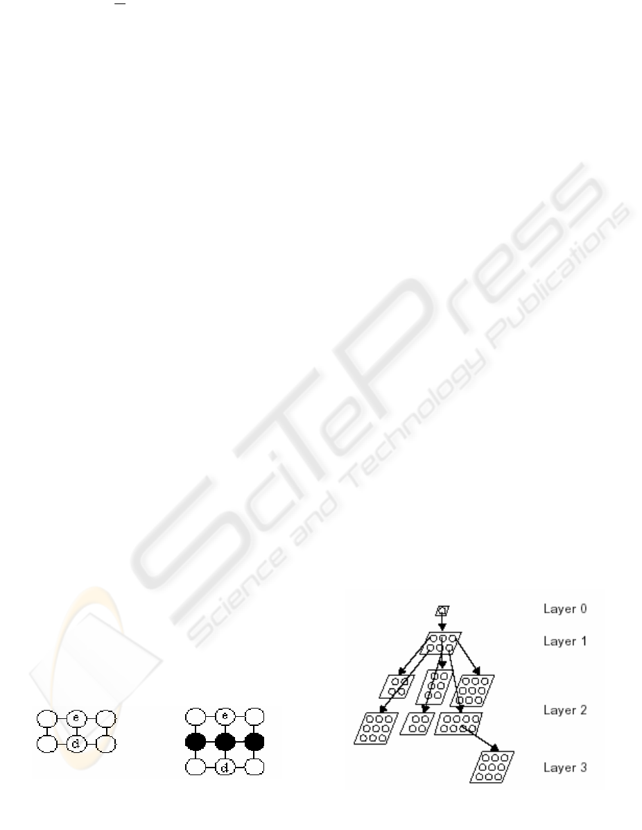
Consider Fig.1 for a graphical representation of the
insertion of units. In this figure the architecture of
the SOM prior to the insertion is shown on the left
hand side where we find a map of 2x3 units with the
error unit labeled by e and its dissimilar neighbor
signified by d. Since the most dissimilar neighbor
belongs to another row within the grid, a new row is
inserted between units e and d. The resulting
architecture is shown on the right hand side of the
figure as a map of now 3 x 3 units.
As soon as the growth process of the first layer map
is finished, i.e. MQE
m
< τ
m
mqe
0
, the units of this
map are examined for expansion on the second
layer. In particular, those units that have a large
mean quantization error will add a new SOM to the
second layer of the GHSOM. The selection of these
units is based on the mean quantization error of layer
0. A parameter τ
u
is used to describe the desired
level of granularity in input data discrimination in
the final maps. More precisely, each unit i fulfilling
the criterion given in expression (4) will be subject
to hierarchical expansion.
∑
=
i
im
mqe
u
MQE
1
(3)
mqe
i
> τ
u
mqe
0
The training process and unit insertion procedure
now continues with these newly established SOMs.
The major difference to the training process of the
second layer map is that now only that fraction of
input data is selected for training which is
represented by the corresponding first layer map
unit. The strategy for row or column insertion as
well as the termination criterion is essentially the
same as used for the first layer map. The same
procedure is applied to any subsequent layers of the
GHSOM.
(4)
The training process of the GHSOM is terminated
when no more units require further expansion. Note
that this training process does not necessarily lead to
a balanced hierarchy, i.e. a hierarchy with equal
depth in each branch. The depth of the hierarchy will
rather reflect the un-uniformity, which should be
expected in real world data collections.
Consider Fig.2 for a graphical representation of a
trained GHSOM. In particular, the neural network
depicted in this figure consists of a single unit SOM
at layer 0, a SOM of 2 x 3 units in layer 1, six SOMs
in layer 2, i.e. one for each unit in layer 1map. Note
that each of these maps might have a different
number and different arrangement of units as shown
in the figure. Finally, there’s one SOM in layer 3,
which was expanded from one of the layer 2 units.
Figure 1: Insertion of units
Figure 2: Architecture of a GHSOM
UNSUPERVISED ARTIFICIAL NEURAL NETWORKS FOR CLUSTERING OF DOCUMENT COLLECTIONS
385
To summarize, the growth process of the GHSOM is
guided by two parameters τ
u
and τ
m
. The parameter
τ
u
specifies the desired quality of input data
representation at the end of the training process.
Each unit i with mqe
i
> τ
u
mqe
0
will be expanded,
i.e. a map is added to the next layer of the hierarchy,
in order to explain the input data in more detail.
Contrary to that, the parameter τ
m
specifies the
desired level of detail that is to be shown in a
particular SOM. In other words, new units are added
to a SOM until the MQE of the map is a certain
fraction, τ
m
, of the mqe of its preceding unit. Hence,
the smaller τ
m
the larger will be the emerging maps.
Conversely, the larger τ
m
the deeper will be the
hierarchy.
3 DATA SET
For the experiments presented thereafter we use a
collection of abstracts from the first International
Conference on Intelligent Computing and
Information Systems, ICICIS 2002.
(
http://asunet.shams.edu.eg/confs/icicis2002.html) as
a sample document archive. ICICIS contains papers
covering the areas of; fuzzy sets, rough sets, genetic
algorithms, neural nets, data mining and knowledge
discovery, expert systems, information storage and
retrieval, web-based learning, medical informatics
and others.
The documents can be thought of as forming topical
clusters in the high-dimensional feature space
spanned by the words that the documents are made
up of. The goal is to map and identify those clusters
on the 2-dimensional map display. Thus we use full-
text indexing to represent the various documents. In
total, ICICIS consists of 68 papers containing 5417
content terms, i.e. terms used for document
representation.
3.1 Document Preprocessing
For the training of SOMs, the documents must be
encoded in form of numerical vectors. To be suited
for the learning process of the map, to similar
documents similar vectors have to be assigned. After
training of the map, documents with similar contents
should be close to each other, and possibly assigned
to the same neuron. The presented approach is based
on statistical evaluations of word occurrences. We
do not use any information on the meaning of the
words since in domains like scientific research we
are confronted with a wide and (often rapidly)
changing vocabulary, which is hard to catch in fixed
structures like manually defined thesaurus or
keyword lists. However, it is important to be able to
calculate significant statistics. Therefore, the number
of considered words must be kept reasonably small,
and the occurrences of words sufficiently high. This
can be done by either removing words or by
grouping words with equal or similar meaning. A
possible way to do so is to filter so-called stop words
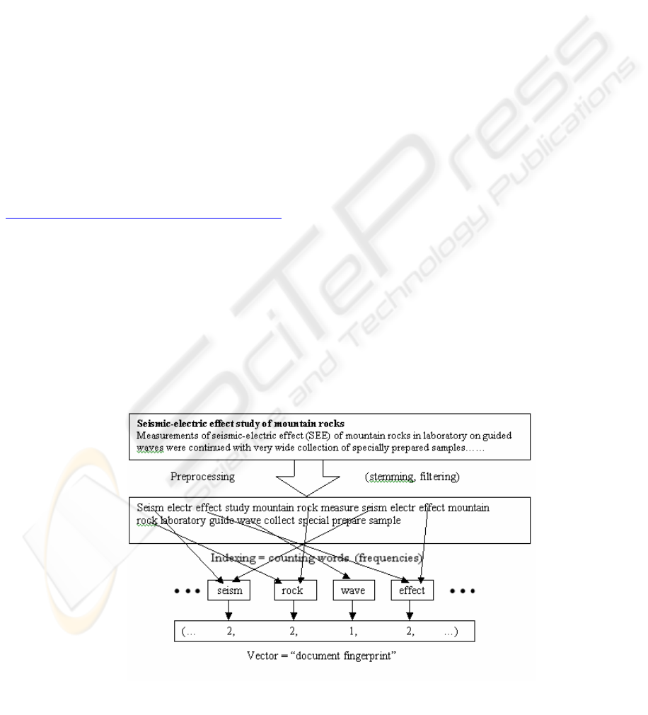
and to build the stems of the words. An overview of
document pre-processing and encoding is given in
Figure 3.
Figure 3: Document preprocessing and encoding
ICEIS 2004 - ARTIFICIAL INTELLIGENCE AND DECISION SUPPORT SYSTEMS
386

The idea of stop word filtering is to remove words
that bear no content information, like articles,
conjunctions, prepositions, etc. Furthermore, words
that occur extremely often can be said to be of little
information content to distinguish between
documents. Also, words that occur very seldom are
likely to be of no particular statistical relevance.
Stemming tries to build the basic forms of words,
i.e. strip the plural ‘s’ from nouns, the ‘ing’ from
verbs, or other affixes. A stem is a natural group of
words with equal (or very similar) meaning. We
currently used the stemming algorithm of (Porter,
1980), which uses a set of production rules to
iteratively transform (English) words into their
stems.
3.2 Generating Characteristic
Document Vectors
Figure 3 shows the principle of the proposed
document encoding. At first, the original documents
are preprocessed, i.e. they are split into words, then
stop words are filtered and the word stems are
generated. The occurrences of the word stems
(frequencies) associated with the document are
counted. A component in a n-dimensional vector is
built, that characterizes the document. These vectors
can be seen as the fingerprints of each document.
For every document in the collection such a
fingerprint is generated. Using GHSOM, these
document vectors are then clustered and arranged
into a 2-dimensional maps, the so-called document
maps. Furthermore, each unit is labeled by specific
keywords that describe the content of the assigned
documents. The labeling method we used is based
on methods proposed in (Lagus et Al., 1999). It
focuses on the distribution of words used in the
documents assigned to the considered unit compared
to the whole document database.
4 EXPERIMENTAL RESULTS
AND DISCUSSION
For our data set we trained both conventional self-
organizing map and growing hierarchical SOM
(GHSOM); to explain the difference and investigate
the benefits of using GHSOM.
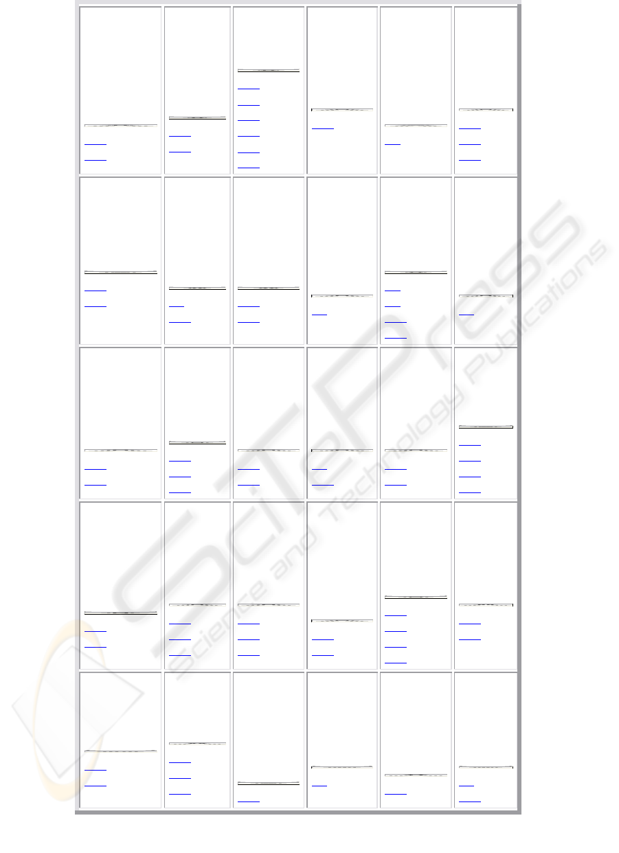
4.1 Trained Conventional SOM
Figure 4 shows a conventional self-organizing map
trained with the ICICIS abstracts data set. It consists
of 5 x 6 units represented as table cells with a
number of abstracts being mapped onto each
individual unit (we refer to the abstract with symbol
T). Each unit is labeled by specific keywords that
describe the content of the assigned abstracts. The
abstracts mapped onto the same or neighboring units
are considered to be similar to each other in terms of
the topic they deal with. We find, that the SOM has
succeeded in creating a topology preserving
representation of the topical clusters of abstracts. For
example, in the lower left corner we find a group of
units representing abstracts on the grid computing.
To name just a few, we find abstracts T22, T23 on
unit (5/1)
1
covering resource scheduling in grid
computing or T51, T53, T68 on unit (5/2) dealing
with intrusion detection architecture for
computational grids. A cluster of documents
covering knowledge discovery and data mining is
located in the upper left corner of the map around
units (1/1) and (1/2), next to a cluster on genetic
algorithms on units (1/3) and (2/3). Below this area,
on units (3/1), (3/2) and neighboring ones we find
abstracts on neural networks. Similarly, all other
units on the map can be identified to represent a
topical cluster of news abstracts.
4.2 Trained GHSOM
Based on the artificial unit representing the means of
all data points at layer 0, the GHSOM training
algorithm started with a 2 x 2 SOM at layer 1. The
training process for this map continued with
additional units being added until the quantization
error fell below a certain percentage of the overall
quantization error of the unit at layer 0. As
mentioned earlier, the growth process of the
GHSOM is guided by two parameters τ
m
and τ
u
. We
can say that, the smaller the parameter value τ
m
, the
more shallow the hierarchy, and that, the lower the
setting of parameter τ
u
, the larger the number of
layers in the resulting GHSOM network will be.
1
We use the notion (x/y) to refer to the unit located
in row x and column y of the map, starting with (1/1)
in the upper
UNSUPERVISED ARTIFICIAL NEURAL NETWORKS FOR CLUSTERING OF DOCUMENT COLLECTIONS
387

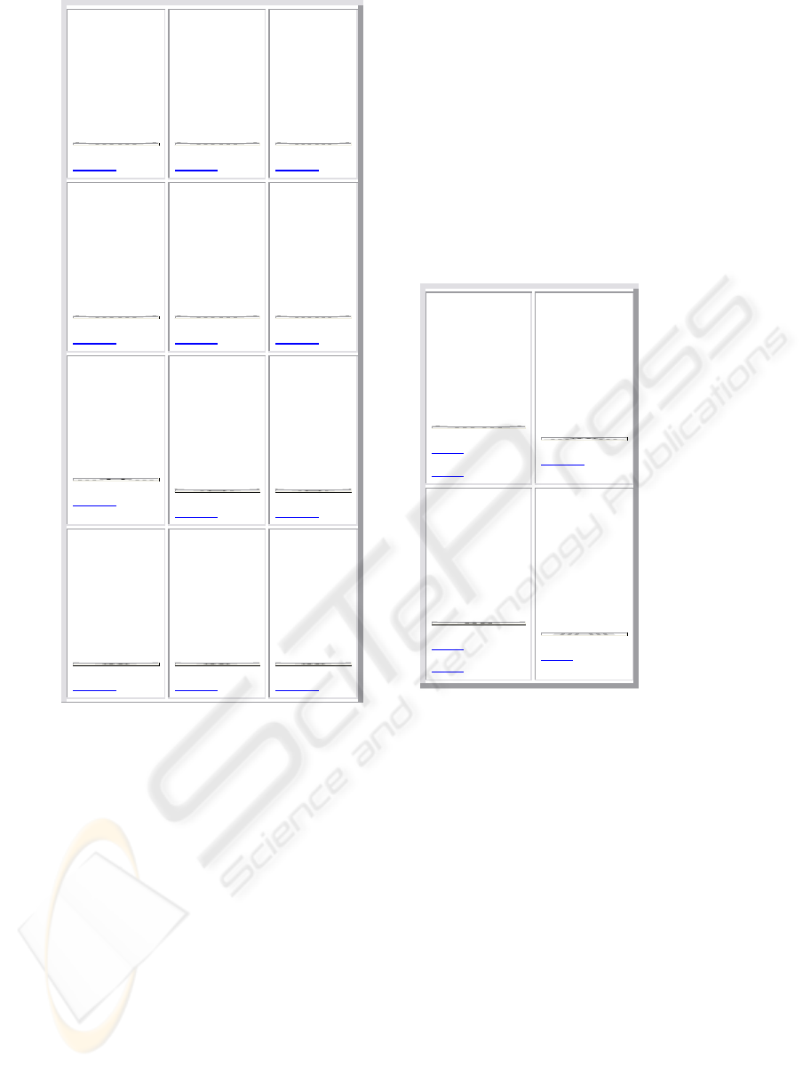
4.2.1 Deep Hierarchy
Training the GHSOM with parameter τ
m
= 0.07 and
τ
u
= 0.0035 results in a rather deep hierarchical
structure of up to 4 layers. The layer 1 map is
depicted in fig. 5(a) grows to a size of 4 x 3 units, all
of which are expanded at subsequent layers. For
convenience we list the topics of the various units,
rather than the individual abstracts in the figure. For
example, we find unit (2/1) to represent all abstracts
related to knowledge discovery and data mining,
whereas neural network topics are covered on unit
(2/2), or abstracts related to genetic algorithms on
unit (4/1) in the lower left corner. Based on this first
separation of the most dominant topical clusters in
the abstract collection, further maps were
automatically trained to represent the various topics
in more detail. This results in 12 individual maps on
layer 2, each representing the data of the respective
higher-layer unit in more detail. Some of the units
on these layer 2 maps were further expanded as
distinct SOMs in layer 3.
We find the branch on data mining on unit (2/1) of
this map. This unit has been expanded to form a 2 x
2 map in the second layer as shown in fig. 5(b). Unit
(1/1) of this map is dominated by abstracts related to
enhancing algorithms for data mining, whereas, for
example, abstracts focusing on mining medical data
set are located in the lower left corner on unit (2/1).
Other dominant cluster on this map is rough set.
One unit of this second layer map is further
expanded in a third layer. Unit (1/2) in the upper
right corner representing abstracts related to data
mining using statistical techniques. These abstracts
are represented in more detail in the third layer.
4.2.2 Shallow Hierarchy
To show the effect of different parameter
settings we trained a second GHSOM with τ
m
set to half of the previous value (τ
m
= 0.035),
while τ
u
, i.e. the absolute granularity of data
representation, remained unchanged. This leads
to a more shallow hierarchical structure of only
up to 2 layers, with the layer 1 map growing to
a size of 5 x 4 units depicted in fig. 6. Again,
we find the most dominant branches to be, for
example, genetic algorithms located on unit
(1/3), data mining and knowledge discovery on
unit (2/3), and neural networks on the lower
right corner of this map. However, due to the
large size of the resulting first layer map, a fine-
grained representation of the data is already
provided at this layer. This results in some
larger clusters to be represented by two
neighboring units already at the first layer,
rather than being split up in a lower layer of the
hierarchy. For example, we find the cluster on
neural networks to be represented by two
neighboring units. One of these, on position (5/3),
covers abstracts related to using neural networks in
the industry. The neighboring unit to the right,
i.e. located on position (5/4) covers other
usages of neural networks.
ICEIS 2004 - ARTIFICIAL INTELLIGENCE AND DECISION SUPPORT SYSTEMS
388
Algorithm
rough
database
knowledge
Mine
T61
T63
Mine
data
system
Intelligent
Discovery
T56
T57
algorithm
genetic
Iris
T15
T32
T35
T37
T39
T60
algorithm
layout
Graph
T19
Approach
paper
Graph
problem
propose
T7
cluster
Mine
algorithm
data
spatial
T55
T58
T59
set
system
attribute
T38
T44
algorithm
time
OAT
Optimum
binary
T9
T65
use
algorithm
genetic
compare
expert
T20
T34
Engine
education
University
course
precious
T5
paper
set
object
include
formula
T1
T3
T13
T17
system
algorithm
Engine
Test
practice
T2
classify
learn
network
neural
rule
T45
T47
detect
system
neural
network
Artificial
T24
T36
T42
net
algorithm
Diffserv
traffic
contour
T11
T12
time
develop
example
paper
deploy
T8
T26
method
control
design
aircraft
require
T10
T30
system
load
distribute
ATM
T18
T21
T25
T49
neural
Model
network
approach
problem
T43
T46
network
Optimum
problem
algorithm
propos
T33
T40
T41
algorithm
interest
wavelet
feature
Arab
T14
T16
T64
query
retrieval
Boolean
translate
Model
T62
T67
logic
uncertainty
Model
inform
mobile
T27
T28
T29
T31
user
design
system
inform
T48
T54
resource
grid
compute
T22
T23
grid
intrusion
process
T51
T53
T68
technology
Egypt
E-
Commerce
inform
Model
T66
field
role
user
technology
T4
system
contain
capacity
section
CBR
T50
system
search
structure
find
custom
T6
T52
Figure 4: 5 x 6 SOM of the ICICIS conference
UNSUPERVISED ARTIFICIAL NEURAL NETWORKS FOR CLUSTERING OF DOCUMENT COLLECTIONS
389
use
result
introduce
Quality
algorithm
down
inform
set
Model
E-business
accid
down
paper
approach
method
design
structure
down
paper
data
system
knowledge
Mine
down
system
learn
network
neural
Artificial
down
paper
use
high
apply
resource
down
network
algorithm
recognize
image
down
set
paper
education
system
web
down
use
ability
database
base
data
down
approach
genetic
propos
problem
algorithm
down
paper
solve
problem
Graph
Optimum
down
select
Draw
represent
algorithm
view
down
4.3 Comparison of Both Models
(Conventional SOM and
GHSOM)
While we find the SOM to provide a good
topologically ordered representation of the various
topics found in the abstracts collection, no
information about topical hierarchies can be
identified from the resulting flat map. Apart from
this we find the size of the map to be quite large
with respect to the number of topics identified. This
is mainly due to the fact that the size of the map has
to be determined in advance, before any information
about the number of topical clusters is available.
GHSOM has two benefits over conventional self-
Mine
data
database
algorithm
Discovery
T56
T57
data
algorithm
classify
system
statistic
down
Mine
medical
data
knowledge
Information
T59
T61
set
knowledge
algorithm
database
rough
T63
(b) Layer 2 map: 2x2 units;
Knowledge discovery
(a) Layer 1 map: 4x3 units; Main topics
Figure 5: Top and second level maps
organizing maps, which make this model
particularly attractive in an information retrieval
setting. First, GHSOM has substantially shorter
training time than self-organizing map. The reason
for that is, there is the obvious input vector
dimension reduction on the transition from one layer
to the next. Shorter input vectors lead directly to
reduced training time because of faster winner
selection and weight vector adaptation. Second,
GHSOM may be used to produce disjoint clusters of
the input data. Moreover, these disjoint clusters are
gradually refined when moving down along the
hierarchy. Contrary to that, the self-organizing map
in its basic form cannot be used to produce disjoint
clusters. The separation of data items is a rather
tricky task that requires some insight into the
structure of the input data. What one gets, however,
ICEIS 2004 - ARTIFICIAL INTELLIGENCE AND DECISION SUPPORT SYSTEMS
390
time
algorithm
Optimum
tree
binary
down
implement
algorithm
perform
Queue
Model
T12
algorithm
approach
problem
genetic
down
approach
query
document
inform
retrieve
down
process
service
efficient
implement
paper
down
paper
traffic
data
GPS
system
down
Mine
data
algorithm
set
knowledge
down
paper
compute
extract
result
match
down
use
Model
technique
process
work
down
control
design
estimate
system
aircraft
down
system
resource
network
compute
apply
down
result
paper
compare
algorithm
down
Model
evolve
software
process
down
variable
determine
classify
rule
system
down
network
propos
grid
describe
study
down
algorithm
interest
Arab
segment
Character
down
system
balance
load
heterogeneous
distribute
down
neural
set
Artificial
system
level
T24
paper
network
neural
operation
level
down
learn
network
neural
regress
recognition
down
Figure 6: Layer 1 map: 5x4 units shallow hierarchy
from a self-organizing map is an overall representation of
input data similarities. In this sense we may use the
following picture to contrast the two models of neural
networks. Self-organizing maps can be used to produce
maps of the input data whereas GHSOM produces an atlas
of the input data. Taking up this metaphor, the difference
between both models is quite obvious. Self-organizing
maps, in our point of view, provide the user with a single
picture of the underlying data archive. As long as the map
is not too large, this picture may be sufficient. As the maps
grow larger, however, they have the tendency of providing
too little orientation for the user. In such a case we would
advise to change to GHSOM as the model for representing
the contents of the data archive. In this case, the data is
UNSUPERVISED ARTIFICIAL NEURAL NETWORKS FOR CLUSTERING OF DOCUMENT COLLECTIONS
391

organized hierarchically, which facilitates browsing into
relevant portions of the data archive.
5 CONCLUSIONS AND FUTURE
WORK
We presented the GHSOM, a novel neural network
model based on the self- organizing map. The main
feature of this model is its capability of dynamically
adapting its architecture to the requirements of the
input space. Instead of having to specify the precise
number and arrangement of units in advance, the
network determines the number of units required for
representing the data at a certain accuracy level at
training time. This growth process is guided solely
by the desired granularity of data representation. As
opposed to other growing network architectures, the
GHSOM does not grow into a single large map, but
rather dynamically evolves into a hierarchical
structure of growing maps in order to represent the
data at each level in the hierarchy at certain
granularity. This enables the creation of smaller
maps, resulting in better cluster separation due to the
existence of separated maps. It further allows easier
navigation and interpretation by providing a better
overview of huge data sets.
We demonstrated that both the self-organizing map
and the hierarchical feature map are highly useful
for assisting the user to find his or her orientation
within the document space. The shortcoming of the
self-organizing map, however, is that each document
is shown in one large map and thus, the borderline
between clusters of related and clusters of unrelated
documents are sometimes hard to find. This is
especially the case if the user does not have
sufficient insight into the contents of the document
collection. The GHSOM overcomes this limitation
in that the clusters of documents are clearly visible
because of the architecture of the neural network.
The document space is separated into independent
maps along different layers in a hierarchy. The
similarity between documents is shown in a fine-
grained level in maps of the lower layers of the
hierarchy while the overall organizational principles
of the document archive are shown at higher layer
maps. Since such a hierarchical arrangement of
documents is the common way of organizing
conventional libraries, only small intellectual
overhead is required from the user to find his or her
way through the document space.
An important feature of GHSOM is that, the training
time is largely reduced by training only the
necessary number of units for a certain degree of
detail representation. The benefits of the proposed
approach have been demonstrated by a real world
application from the text classification domain.
Our future work on GHSOM includes fine-tuning
the basic algorithm and applying it to collections in
any language, provided that words as primary tokens
can be identified. This may require special
preprocessing steps for languages as Chinese, where
word boundaries are not eminent from the texts. In
addition, develop a method for setting the threshold
values (τ
m
and τ
u
) automatically according to
application requirements.
REFERENCES
T. Kohonen, “Self-organized formation of topologically
correct feature maps,” Biol. Cybern. vol. 43, 1982,
pp. 59–69.
T.Kohonen, “Self-organizing maps” Berlin, Germany:
Springer verlage, 1998.
K. Lagus, T. Honkela, S. Kaski, and T. Kohonen, “Self-
organizing maps of document collection: A new
approach to interactive exploration” In Proc. Int.
Conf. on Knowledge Discovery and Data Mining
(KDD-96), Portland, OR, vol.36, 1998, pp. 314-322
D. Merkl, “Exploration of text collections with
hierarchical feature maps”. In Proc. Int. ACM
SIGIR Conf. on Information Retrieval (SIGIR'97),
Philadelphia, PA, vol.62, 1997,pp. 412-419
A. Rauber and D. Merkl, “Finding structure in text
archives” In Proc. Europe an Symp. on Artificial
Neural Networks (ESANN98), Bruges, Belgium,
vol.18, 2000,pp.410-419
B. Fritzke, “Growing self-organizing networks -------
Why?” In Proc. Europ Symp on Artificial Neural
Networks (ESANN'96), Bruges, Belgium,
vol.16,1998,pp.222-230.
B. Fritzke, “Growing grid: a self-organizing network
with constant neighborhood range and adaptation
strength” Neural Processing Letters, 1997.
R. Miikkulainen, “Script recognition with hierarchical
feature maps” Connection Science, 2, 1995.
M. Salem, M. Syiam, and A. F. Ayad, “Improving self-
organizing feature map (SOFM) training algorithm
using k-means initialization” In Proc. Int. Conf. on
Intelligent Eng. Systems INES, IEEE,
vol.40,2003,pp.41-46.
M. Porter, “An algorithm for suffix stripping” Program
14(3), pp. 130-137, 1980.
K. Lagus, and S. Kaski, “Keyword selection method for
characterizing text document maps” In Proc of
ICANN99, Ninth International Conference on
Artificial Neural Networks,IEEE,vol 68, 1999,pp.615-
623
ICEIS 2004 - ARTIFICIAL INTELLIGENCE AND DECISION SUPPORT SYSTEMS
392
