A COMPARISON BETWEEN THE PROPORTIONAL KEEN

APPROXIMATOR AND THE NEURAL NETWORKS LEA

RNING

METHODS

Peyman Kabiri

College of Computer Engineering, Iran’s University of Science and Technology, Narmak, Tehran, Iran

eywords: Machine Learning, Data Visualisation and Approximation.

Abstract: The Proportional Keen Approximation method is a young learning method using the linear approximation to

learn hypothesis. In the paper this methodology will be compared with another well-established learning

method i.e. the Artificial Neural Networks. The aim of this comparison is to learn about the strengths and

the weaknesses of these learning methods regarding different properties of their learning process. The

comparison is made using two different comparison methods. In the first method the algorithm and the

known behavioural model of these methods are analysed. Later, using this analysis, these methods are

compared. In the second approach, a reference dataset that contains some of the most problematic features

in the learning process is selected. Using the selected dataset the differences between two learning methods

are numerically analysed and a comparison is made.

1 INTRODUCTION

In a research aimed to compensate for the errors due

to the flexibility and the backlash in mechanical

systems (Kabiri, 2002), and after unsuccessful

implementation of the Artificial Neural Networks

(ANN), attention was focused on finding a more

suitable method. By the ANN, the author means the

Back Propagation (BP) model of the ANN. The aim

for that research was to compensate for the

positioning errors of a robotic arm by considering it

as a Black Box (Mingzhong, 1997). After much

research using linear approximation methodology a

novel machine learning method was developed and

implemented (Kabiri, 1998 & 1999). This approach

provides the adaptability feature for the controller

but requires a large population of samples. The need

for simplicity in the data set might be the reason

why previously the researchers were only using this

approach for the joints of the manipulator (Chen,

1986). Main problems with the ANN were its slow

training and difficulty in training it with complicated

patterns in the dataset (Kabiri, 1998)(Sima, 1996).

Once the population of the dataset increases, these

problems will get worse. The Proportional Keen

Approximator (PKA) has no training stage as in the

ANN and at the most problematic areas for the ANN

it can work without any problems. On the other hand

this method has some limitations of its own, some of

which might be handled in future e.g. requires more

memory than the ANN and needs tabulated sampled

dataset. As it will be described in the following

section the early version of the PKA was introduced

in the Cartesian co-ordinate system (Kabiri, 1998).

The basic cell had two inputs and one output. Later a

new version with three inputs and one output was

introduced. Currently the work is being continued to

extend the PKA into the Spherical and Cylindrical

co-ordinate systems that will broaden its scope of

application. The PKA in the Cartesian co-ordinate

system is implementing the linear approximation to

interpolate between the sample points. The PKA is a

Memory-Based Learning (MBL) system and

requires large memory capacity (Schaal, 1994).

At the following sections the reader will first

learn about the PKA methodology. The properties of

these methods are compared both in numerical and

descriptive ways. Using a sampled dataset derived

from an equation, the ANN and the PKA

methodologies are compared numerically against

each other and results are presented.

159

Kabiri P. (2004).

A COMPARISON BETWEEN THE PROPORTIONAL KEEN APPROXIMATOR AND THE NEURAL NETWORKS LEARNING METHODS.

In Proceedings of the Sixth International Conference on Enterprise Information Systems, pages 159-164

DOI: 10.5220/0002599401590164

 SciTePress

2 2D-PKA IN CARTESIAN CO-

ORDINATES SYSTEM

This Approximator is designed for 2 input and 1

output configuration (2D). Later it was expanded to

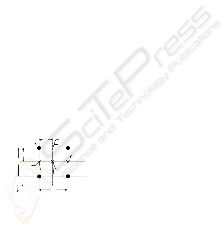
3 input and one output configuration (3D). In the 2D

configuration as it is illustrated in Figure 1, for every

ordered pair of (x, y) in the function domain, output

of the system can be calculated considering three

conditions:

Condition 1. Both of the x and y are available in

the sampled data set area. In this condition, the

output will be the actual given data sample.

Therefore, the accuracy is matched by default 100%

e.g. A (x

, y

, z

) in Figure 1.

Condition 2. One of the input components (x or y)

overlays one of the Rows or Columns in the given

data sample. If the given point has either of the x or

y components equal to one of the components of the

sampled data, this condition will be triggered. For

example, if the ordered pair of (x, y) is considered as

input and z considered as the data component that

determines the amount of error in that location. The

output is calculated with respect to two adjacent

neighbours of the given point. Only values of the

two unequal components (in the sample and the

given data pairs) are used for the calculations. For

example, let

xx = for the pairs (x

, y

) and (x

). Then for calculating the output only the y

components are used. e.g.

B (x

+∆x, y

, z

) when

xx = and

C (x

, y

+∆y, z

) when

yy = .

Condition 3. None of the input co-ordinates are

equal to any of the Rows or Columns in the

Approximator. In this condition the method will be

applied to one of the components (x or y) first. Then

the result of the calculation is used for the

proportional approximation on the other pair of

components (same as condition 2). In this condition

the output value is calculated by D (x

+∆x, y

+∆y,

) i.e. output = z

in Figure 1.

3 METHODOLOGY OF 3D-PKA

The main difficulty for understanding the 3D-PKA

is the visualisation of the method that is going to be

explained at the following. The key point to

understand the idea of expanding the PKA into the

dimension is to consider each 2D-PKA as a plane

surface. Here instead of points, flat surfaces are

considered and the rest is similar to the 2D-PKA

(Kabiri, 1999). Figure 2 illustrates the concept. A

point can either be on the top or the bottom layer, or

it can be between the two layers. In the first two

cases the estimated value is the returned value from

the 2D-PKA cell (either the top or the bottom layer

that holds the point) i.e. Condition 1. However for

the third case the estimated value is the result of a

linear approximation between the results out of both

top and bottom 2D-PKA layers i.e. Condition 2. It

should be noted that as the number of dimensions

increases, the required computation power for the

method increases as well. The same is with the

memory requirements for the 3D-PKA.

4 PROPERTIES OF THE PKA

In the ANN the number of links and nodes in the In

the ANN the number of links and nodes in the

network depends on the complexity of the training

data set. Therefore the execution speed for the ANN

is directly related to the complexity of the training

data set. However, only one PKA cell is required to

learn the pattern regardless of the complexity of the

sampled data set. This means that in the PKA

method, speed is independent from the complexity

of the sampled data set. Since the number of

operations in this method is smaller and due to the

simplicity of these operations

, the PKA in the

forward execution needs less calculation power than

the other alternative methods such as the ANN

(particularly in 3D). In the worst case scenario

∆

r and c are Row and Column

, z

, and z

are values of the sampled points where

()()

Lxzzzz /*

121

∆−+= ,

()()

Lyzzzz /*

131

∆−+= ,

()()

Lyzzzz /*

2422

∆−+= , and

()()

xCCCD

Lxzzzz /*

∆−+= ; are calculated values.

Figure 1: Calculation Method for the 2D-PKA

Approximator

ICEIS 2004 - ARTIFICIAL INTELLIGENCE AND DECISION SUPPORT SYSTEMS

160

(condition 3) every 2D-PKA cell needs 3 addition, 6

subtraction, 3 multiplication and 3 division operation

times plus the time needed for the memory address

calculation and data fetching (delays due to memory

related operation are assume to be constant).

However, for the ANN this time varies with the size

of the network (considering an operation time of one

+or- operation time for every node and an operation

time of one *or/ operation for each link). Therefore

the PKA in the forward execution is expected to be

faster than medium or large size ANN. Of course the

actual difference depends on the specific ANN and

needs to be quantified for each individual case. As

an example, a fully connected and biased ANN with

the 2:11:15:1 structure can be considered for

comparison where 229 multiplication operations and

202 (2-input addition) operations are required

(Kabiri, 1999).

Approximator has three levels of precision. As

explained above, accuracy in the first condition is

100%. The second and the third conditions

respectively have less accuracy. The amount of error

in the two latter conditions depends on the closeness

of the graph between two sample points to the

straight line. The amount of error in those conditions

also relates to the distance between two sample

points. This means that the higher the resolution, the

more accurate is the approximation. There is no

training stage for this approach and it is ready as

soon as all the samples become accessible to the

Approximator (Loaded into the memory). Despite

the complexity of the pattern introduced to the PKA,

one PKA cell is sufficient for learning the pattern.

Another feature for this method is the possibility to

update the knowledge of the PKA while using it.

This is because the database generated by the

method (tabular data), enables us to accurately

locate any part of the knowledge and change it.

5 RESULTS

In order to perform a numerical comparison between

the PKA and the ANN methodologies an experiment

is prepared. In this experiment the data derived from

an equation is used as a frame of reference and the

methodologies were compared with respect to this

frame of reference. In the following, the experiment

is described and results are presented.

5.1 System Variables

As it is described in section 4 the accuracy for the

PKA in sampled points is 100%. Therefore, the

Maximum Error and the Mean Square Error (MSE)

for the PKA at the sampled points are zero. In order

to compare the PKA with the ANN method the

following experiment was designed and

implemented (Kabiri, 1999).

This experiment is aimed to help both in

comparing the important features in the hypothesis

surfaces of these methods and their resultant error

values. These methods (ANN and PKA) will be

compared with respect to the error values resulting

in the sampled points, interim points and finally all

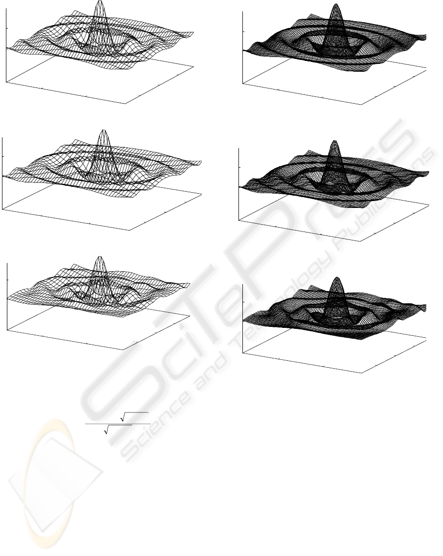
together. In order to do the comparison, function

()

(

)

sin*0.100

vuSINC

was selected as the

frame of reference for the comparison, because it is

sufficiently complex to include a range of angular

variations from very sharp to gently curved patterns.

The properties of this function are analysed to

provide a better form of comparison. The original

domain of the

()

vuSINC ,

function is

[]

2/2/,

ππ

−∈vu

. The input domains for the

function are moved to

[]

0.2450.110∈x

and

[]

0.900.90−∈y

in the scale of millimetres. The

maximum value for the function is 100.0mm. Using

this function, a sample dataset was produced in

equal sampling steps of 3.0mm for the x-axis and

9.0mm for the y-axis. The ANN was trained using

the generated dataset. As the PKA method has no

training stage, it uses this dataset for the

generalisation.

In order to generate the generalised dataset, the

sampling step for the x and y-axes were respectively

altered to 1.0mm and 3.0mm. In other words the

resolutions for the axes are increased by the factor of

3. The total number of samples introduced to both

methods is 966 samples. As the result of the

generalisation, the population of the sampled dataset

increases to 8296 samples. The following describes

Condition 1

Condition 2

2D-PKA

Top Layer

2D-PKA

Bottom Layer

Figure 2: Methodology for the 3D-PKA Calculations.

1. Simpler operation means shorter execution time for the operation.

A COMPARISON BETWEEN THE PROPORTIONAL KEEN APPROXIMATOR AND THE NEURAL NETWORKS

LEARNING METHODS

161

the training parameters of the ANN.

The ANN consists from a fully connected and

biased with 2 layers network structure of 2:11:15:1.

The training for the ANN was carried out on a

Pentium-400 based PC. Learning rate was initially

equal to 0.9 and later it was changed to 0.7, 0.5, 0.3,

0.2 and 0.1. Momentum factor for the training was

0.9 and was later changed to 0.8 and finally 0.7. The

training was many times forced to restart again. This

was because of different reasons such as need for

more nodes in the network, over training or lack of

progress in the training. The training process took

around 10 days. In the final reported training, the

total number of elapsed epochs was 1382755

epochs. Total training time was 285899.0 seconds

(3 days, 7 hours, 24 minutes and 59 seconds). The

final MSE using normalised data on the output was

0.00027 and the final MSE using de-normalised (in

order to make it comparable with the PKA values)

data on the output was 6.04.

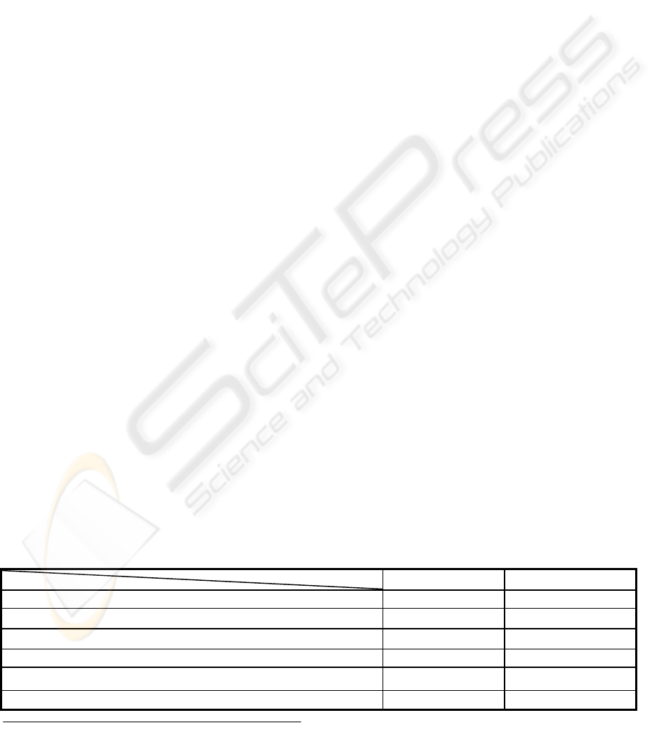
Table 1 compares two methods. In this table by

the term “the whole generalised points” the author

means the sampled points plus the generalised

interim points. Figure 4-a to Figure 4-c respectively

depict the output from the reference equation, PKA

and ANN. In Figure 3-a to Figure 3-c the

aforementioned dataset is generalised using

respectively the reference equation, PKA and ANN.

In analysing the data it is important to

understand that in any estimation the size of the

sampling step plays an important role in the final

resulting estimation error. If the speed of change in

the dataset is very high then a small sampling step is

required. This is some how the case in this example.

The ratio of the rise in the height of the graph is

sometimes too fast for the applied sampling step

size. Figure 5 depicts this concept.

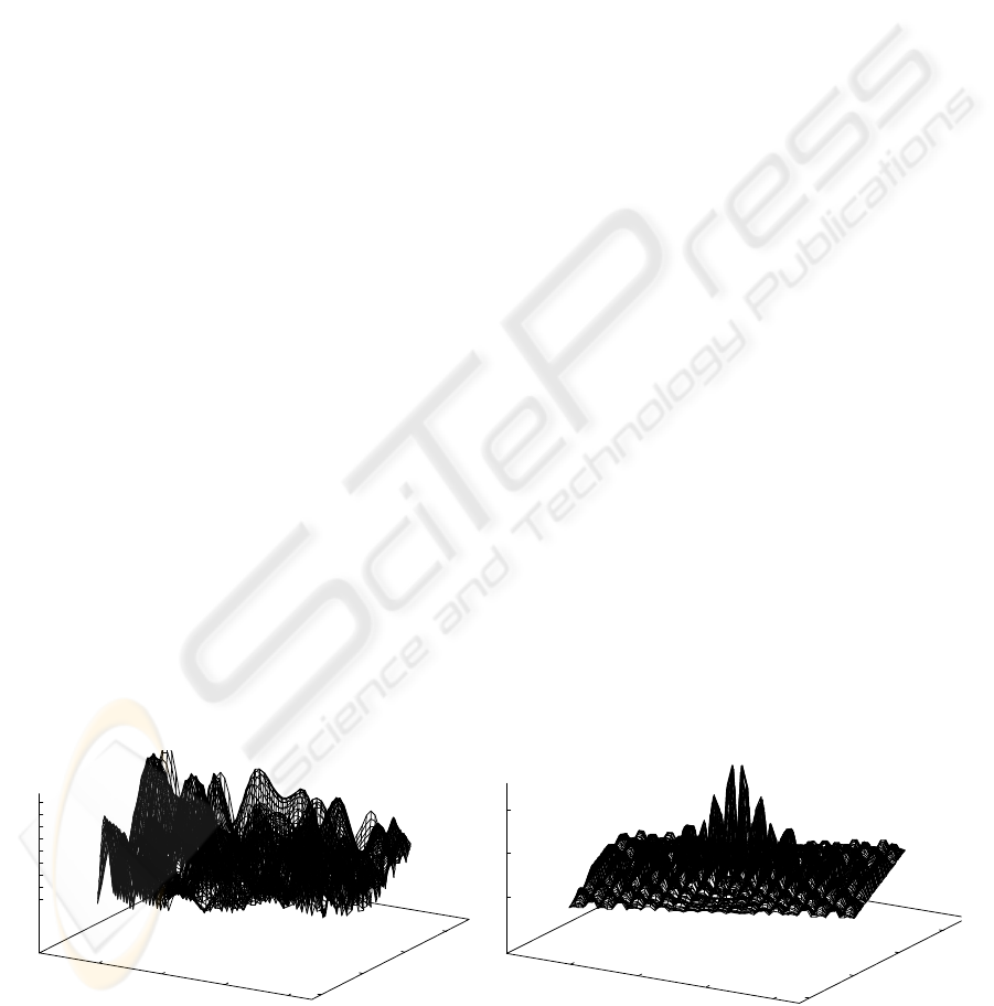
As it can be seen in Figure 5-a, in the PKA

method the error values are higher at the centre of

the function domain than the rest of the points. In the

PKA method, the error is not evenly distributed in

the function domain. In this example in the PKA

method, although the maximum error seems to be

higher than the ANN method (Figure 5-b), most of

the points are well below the MSE value.

Figure 5-b depicts the distribution of the error

values in the ANN method. This figure shows that

the ANN method has a more evenly distributed error

pattern than the PKA method. However most of the

error values in this method are close to its MSE.

5.2 Analysis of the Result

Analysing the result, first the differences can be

divided into two categories training stage and the

execution stage. Later both of these categories will

be divided into smaller subsets such as difference in

execution speed, accuracy and some differences due

to the properties of the PKA methodology.

In the training stage as it is for the ANN, the

difference is huge. No training for the PKA in

comparison to the 3 days training for the ANN is a

clear advantage for the PKA methodology. Contrary

to the ANN that the required time for the training

can be different from one dataset to another, the time

required for the PKA to learn knowledge (the

training stage) is always the same. This property

plus ability to update the knowledge during the

execution are two of the main advantages of the

PKA. On the other hand PKA requires a large

memory to hold the samples that makes it a

memory-bound process, the fully connected and

biased ANN using the BP model is mostly a CPU-

bound process. Currently cost of the CPU time and

the Memory module are falling.

Sensitivity to the complexity in the training

pattern and sample population affects the training

stage for the ANN and in the supervised training it

might be necessary to reorganise the network and

restart the training. However, in the PKA none of

these problems will be encountered. After the

training for the ANN using extra sample points the

result has to be verified, but in the PKA due to the

consistency in the linear approximation this is not

necessary. In the reported experiment maximum

error in the PKA method was larger than the ANN

method. This difference is due to the large

Table

: A numerical comparison between the PKA and the ANN. All the values are in millimetres

(MSE is

calculated using de-normalised data values). (*) Means that: Where output should be 91.98 it was 78.95

The ANN The PKA

Maximum

error for the sampled points. 1.3 0.0

MSE for the sampled points. 6.0 0.0

Maximum error (difference) for the interim points. 8.7 13.0 (*)

MSE for the interim points. 9.0 4.1

Maximum error (difference) for the whole generalised points. 8.7 13.0 (*)

MSE for the whole generalised points. 8.0 3.6

. Maximum error is a relati

ve error (between the reference

value and the generalised value.

ICEIS 2004 - ARTIFICIAL INTELLIGENCE AND DECISION SUPPORT SYSTEMS

162

non-linearity in the hypothesis space at that point

and low sampling step.

This result may change for other curves and it is

an uncertain region for both methods. Nevertheless

this problem is the subject for further research to

implement the PKA method in the Spherical or

Cylindrical co-ordinate systems. In training the

ANN any randomly collected sample data is

acceptable, but the PKA method can only work with

tabulated dataset collected with equal sampling

steps. This is a major drawback for this method, but

the reader has to note that in the industry tabulated

data sampling is the most common method. The

requirement for the tabulated data makes the PKA

not suitable for the biological kind of research

activities that may need to use randomly collected

data. Possibility of using the random sampled data

for the PKA is also a research subject that is under

investigation.

The execution speed of the ANN is dependent on

the organization of the network and the number of

nodes and links in the network. However, the

execution time for the PKA has a maximum delay

condition (Condition 3, section 2 for the 2D-PKA

and section 3); this is because only one cell is

sufficient to learn any complex pattern in the dataset.

150

200

-50

X Axis

Y Ax

Z Axis

a) The original sampled d

ataset with 3 times higher

sample resolution in either of the axes.

150

200

-50

X Axis

Y Axis

Z Axis

The output from the PKA with 3 times higher

sample resolution in either of the axes.

150

200

-50

X Axis

Y Ax

Z Axis

c) The output from the ANN with 3

times higher

sample resolution in either of the axes.

Figure 3: A comparison between the original sampled

dataset and the resulted output from both PKA and ANN

methods with generalisation (X*3, Y*3). The z-axis

represents the output.

150

200

-50

X Axis

Y Axis

Z Axis

a) The original sampled dataset (X*1, Y*1).

150

200

-50

X Axis

Y Axis

Z Axis

b) The output from the PKA with no generalisation.

150

200

-50

X Axis

Y Axis

Z Axis

c) The output from the ANN with no generalisation.

Figure 4: A comparison between the Original sampled

dataset and the resulted output from the both PKA and

ANN methods without any generalisation (X*1, Y*1).

The z-axis represents the output.

()

(

)

sin*0.100

vuSINC

A COMPARISON BETWEEN THE PROPORTIONAL KEEN APPROXIMATOR AND THE NEURAL NETWORKS

LEARNING METHODS

163

Execution time for large and medium size ANN is

longer than the PKA (section 4).

6 CONCLUSIONS

In comparing the PKA and the ANN methodologies,

before deriving any conclusions the reader should be

reminded that in this paper a young (4 years old)

method i.e. PKA has been compared with a well

established method such as the ANN. Therefore,

expectation should be as far as a 4 years old

methodology and one should just consider this

comparison as an introduction to potentials of a new

methodology (PKA) and in no way as a mean of

disregarding the ANN. For the PKA there is still a

long way to go to reach maturity in concept as it has

been achieved for the ANN.

This paper highlights the differences between the

PKA and the ANN methodologies and compares

some limitations of one versus advantages of the

other. In this report only a 2D-PKA in Cartesian co-

ordinates is compared with back propagation type of

the ANN with 2 inputs and 1 output. In both

methodologies sampling resolution plays a major

role in the accuracy of the estimation. In some areas

such as the training process, execution speed and

accuracy the 2D-PKA shows some advantages over

the ANN. On the other hand the ANN has some of

its own properties such as the ability to learn

randomly collected dataset, which the 2D-PKA is

not yet capable of performing. As a young

methodology the PKA still needs more research to

be done to extend its methodology and to find more

about its properties. New generations of the PKA in

Cylindrical and Spherical co-ordinate systems are

expected to provide us with new features and better

accuracy for the estimation of the curved patterns.

REFERENCES

Kabiri, P., 2002. Using Black Box and Machine Learning

Approach in Controlling a Machine. In SMC’02, 2002

IEEE International Conference on Systems, Man and

Cybernetics. IEEE.

Kabiri, P., Sherkat, N. and Shih, V.,1999. Compensating

for Robot Arm Positioning Inaccuracy in 3D-Space, In

SPIE's International Symposium on Intelligent Systems

in Design and Manufacturing II, SPIE.

Kabiri, P., Sherkat, N. and Shih, V.,1998. Compensation

for Robot Arm Flexibility Using Machine Intelligence,

In SPIE's International Symposium on Intelligent

Systems in Design and Manufacturing, SPIE.

Mingzhong, L. and Fuli W., 1997. Adaptive Control of

Black-Box Non-Linear Systems Using Recurrent

Neural Networks, In Proceedings of the 36th IEEE

Conference on Decision and Control, IEEE.

McLauchlan, R. A., Ngamsom, P., Challoo, R. and

Omar S. I., 1997, Three-Link Planar Robotic Arm

Trajectory Planning and Its Adaptive Fuzzy Logic

Control, In IEEE International Conference on Systems

Man and Cybernetics, IEEE.

Sima, J., 1996. Back-propagation is not efficient, In

Neural Networks Journal.

Chen, J. and Chao, L. M., 1986. Positioning Error

Analysis for Robot Manipulators with All Rotary

Joints, Proceedings of IEEE International Conference

on Robotics and Automation, IEEE.

Schaal, S. and Atkeson, C. G., 1994. Robot

Joggling: Implementation of Memory Based

Learning, In IEEE Control Systems, IEEE.

100

150

-250

-200

-150

-100

X A x is

Y Axis

Z Axis

100

150

-250

-200

-150

-10

X Axis

Y Ax

Z Axis

The distribution of the error for the ANN The distribution of the error for the PKA

Figure 5: A comparison for the resultant error between the original sampled dataset and the resulted output from the both

PKA and ANN methods with generalisation (X*3, Y*3). The z-axis represents the difference between the output from the

reference equation (SINC) and the output produced by each method.

ICEIS 2004 - ARTIFICIAL INTELLIGENCE AND DECISION SUPPORT SYSTEMS

164