ANALYSIS OF THE ITERATED PROBABILISTIC WEIGHTED K
NEAREST NEIGHBOR METHOD, A NEW DISTANCE-BASED
ALGORITHM
J. M. Mart
´
ınez-Otzeta and B. Sierra
Dept. of Computer Science and Artificial Intelligence
University of the Basque Country
P.O. Box 649
20080 San Sebasti
´
an, Spain
Keywords:
Supervised Classification, Nearest Neighbor, k-NN, Machine Learning, Pattern Recognition.
Abstract:
The k-Nearest Neighbor (k-NN) classification method assigns to an unclassified point the class of the nearest
of a set of previously classified points. A problem that arises when aplying this technique is that each labeled
sample is given equal importance in deciding the class membership of the pattern to be classified, regardless
of the typicalness of each neighbor.
We report on the application of a new hybrid version named Iterated Probabilistic Weighted k Nearest Neigh-
bor algorithm (IPW-k-NN) which classifies new cases based on the probability distribution each case has to
belong to each class. These probabilities are computed for each case in the training database according to the
k Nearest Neighbors it has in this database; this is a new way to measure the typicalness of a given case with
regard to every class.
Experiments have been carried out using UCI Machine Learning Repository well-known databases and per-
forming 10-fold cross-validation to validate the results obtained in each of them. Three different distances
(Euclidean, Camberra and Chebychev) are used in the comparison done.
1 INTRODUCTION
The nearest neighbor classification method assigns to
an unclassified point the class of the nearest among
a set of previously classified points. This rule is in-
dependent of the underlying joint distribution on the
sample points and their classifications. An extension
to this approach is the k-Nearest Neighbor (k-NN)
method, in which classification is made taken into ac-
count the k nearest points and classifying the unclas-
sified point by a voting criteria among this k points.
We present a new voting method which takes into ac-
count the fact that not all the cases in the database
are typical representatives of the class they belong
to (i.e., they could have some degree of excepcional-
ity). This new method gives to each point in the train-
ing database a measure of its typicality regarding its
neighbors and their typicality as well.
The undergone experimentation suggests that this
new approach improves k-NN results in most of the
databases tested.
The structure of this paper is as follows. The new pro-
posed method is introduced in section 2, as well as a
brief description of k-NN and Probabilistic Weighted
k Nearest Neighbor (PW-k-NN) methods. In section
3 we show the experimental results obtained and in
final section 4 concluding remarks are given.
2 THE ITERATED
PROBABILISTIC WEIGHTED K
NEAREST NEIGHBOR
METHOD (IPW-k-NN)
In this section the new proposed approach is presented
as a new member of the distance based classification
algorithms family. In order to introduce it, we present
first the well known k-NN paradigm, then an exten-
sion of it that weights the neighbors with their prob-
ability of belonging to its class, and finally the new
propossed approach IPW-k-NN is introduced.
2.1 The K-NN Method
A set of pairs (x
1
, θ
1
), (x
2
, θ
2
), ..., (x
n
, θ
n
) is given,
where the x
i
’s take values in a metric space X upon
which is defined a metric d and the θ
i
’s take values
233
M. Martínez-Otzeta J. and Sierra B. (2004).
ANALYSIS OF THE ITERATED PROBABILISTIC WEIGHTED K NEAREST NEIGHBOR METHOD, A NEW DISTANCE-BASED ALGORITHM.
In Proceedings of the Sixth International Conference on Enterprise Information Systems, pages 233-240
DOI: 10.5220/0002605402330240
Copyright
c
 SciTePress

in the set {1, 2, ..., M} of possible classes. Each
θ
i
is considered to be the index of the category to
which the ith individual belongs, and each x
i
is the
outcome of the set of measurements made upon that
individual. We use to say that ”x
i
belongs to θ
i
”
when we mean precisely that the ith individual, upon
which measurements x
i
have been observed, belongs
to category θ
i
.
A new pair (x, θ) is given, where only the mea-
surement x is observable, and it is desired to estimate
θ by using the information contained in the set of
correctly classified points. We shall call
x
0
n
∈ {x
1
, x
2
, ..., x
n
}
the nearest neighbor of x if
min d(x
i
, x) = d(x
0
n
, x) i = 1, 2, ..., n
The Nearest Neighbor (NN) classification decision
method gives to x the category θ
0
n
of its nearest
neighbor x
0
n
. In case of tie for the nearest neighbor,
the decision rule has to be modified in order to break
it. A mistake is made if θ
0
n
6= θ. An straightfor-
ward extension to this decision rule is the so called
k-NN approach (Cover and Hart, 1967), which
assigns to the candidate x the class which is most
frequently represented in the k nearest neighbors to x.
Much research has been devoted to the k-NN rule
(Dasarathy, 1991). We could give different weights to
the variables in the distance computation, or different
weights to each neighbor in the voting process. This
last approach has been developed in the Probabilistic
Weighted k Neighbor Method.
2.2 The Probabilistic Weighted K
Nearest Neighbor Method
(PW-k-NN)
In the k-NN algorithm each of the labeled samples
is given equal importance in order to decide the
class membership of the pattern to be classified,
regardless of their ”typicalness”. Taking into account
this fact, another approach might estimate each case’s
probability of belonging to its real class.
Sierra and Lazkano (Sierra and Lazkano, 2002)
described a k-NN variation, the so called Probabilistic
Weighted k Nearest Neighbor Method (PW-k-NN).
In their work they use Bayesian Networks (Cowell
et al., 1999) to estimate the probability distribution
each case has of belonging to each class.
They use a Bayesian Network learned for classifi-
cation task (Sierra and Larra
˜
naga, 1998) among the
predictor variables selected by a forward simple se-
lection technique (Inza et al., 2000), and present a
new voting method which takes into account the fact
that not all the cases of the database are typical in the
class they belong to. This new method gives to each
point in the training database a measure of its typical-
ity by using the learned Bayesian Network.
2.3 The Iterated Probabilistic
Weighted K Nearest Neighbor
Method (IPW-k-NN)
Our method is a new version of the Probabilistic
Weighted k Nearest Neighbor Method, described
in the previous section. Instead of using Bayesian
Networks to estimate the probabilities, we take into
account the nearest neighbors.
In a first step we estimate how typical is a case
in its own class. This estimation is performed
taken into account a number K
p
of neighbors.
Such estimation is stored in a bidimensional array
P
xy
, x = 1 . . . n, y = 1 . . . M, where P
ij
stands for
the probability that the case i belongs to class j. In
each iteration (the number of iterations is given by
a parameter called β), we compute the new value
of each P
ij
as a combination of the old value and
an estimated P
0
i
j
. A parameter called α determines
the relative weight of these two values in the new
P
ij
. If, for example, provided K
p
= 10, and five
neighbors of case i belong to class θ
1
, four to class
θ
2
and the last one to class θ
3
, we obtain, in a first
step, that P
i1
= 0.5, P
i2
= 0.4 and P
i3
= 0.1. In
further iterations, the new value of P
ij
is computed
as P
ij
← αP
0
i
j
+ (1 − α)P
ij
, where the weight of
the former value of P
ij
as well as P
0
i
j
are weighted.
When the first iteration has finished, each case in the
training database has been associated to a probability
array, which is, in its turn, used to compute P
0
i
j
in
following iterations.
In the second and last step a test case is classified
according to their K
c
neighbors. K
p
1
and K
c
2
may
be differents, because K
p
is used to compute class
probabilities in the training set and K
c
to classify a
test case.
The class which outputs IPW-k-NN for the case i is
the class for which
P
K
c
z=1
P
zi
is maximum.
The new proposed method, IPW-k-NN is shown in its
1
K
p
stands for K neighbors in probability estimation
task
2
K
c
stands for K neighbors in classification task
ICEIS 2004 - ARTIFICIAL INTELLIGENCE AND DECISION SUPPORT SYSTEMS
234

begin IPW-k-NN
As input we have the samples file TR, containing
n cases (x
i
, θ
i
), i = 1, ..., n,
the value of K
p
K
c
, α and β
and a new case (y, θ) to be classified
θ ranges over m classes
FOR each case (x
i
, θ
i
) in TR DO
BEGIN
Search the k Nearest Neighbors of (x
i
, θ
i
)
in TR - (x
i
, θ
i
)
and store their TR index in Neigh
ij
, j = 1, ..., K
p
Initialize the probability array P
ij
associated
to the case i as follows:
if θ
i
= j then P
ij
← 1
otherwise P
ij
← 0
END
FOR β iterations DO
BEGIN
FOR each case (x
i
, θ
i
) in TR DO
BEGIN
Modify the associated probability array P
ij
as follows:
P
0
i
j
← (
P
K
p
z=1
P
Neigh
iz
j
)/K
p
P
ij
← αP
0
i
j
+ (1 − α)P
ij
END
END
Search the K
c
Nearest Neighbors of (y, θ) in TR
Reset the weights of all existing classes W C
i
= 0
FOR each of the k-NN (x
k
, θ
k
) DO
BEGIN
FOR each class i actualize its weight W C
i
as follows:
W C
i
← W C
i
+ P
ki
END
Output the class θ
i
with greatest weight W C
i
end IPW-k-NN
Figure 1: The pseudo-code of the Iterated Probabilistic
Weighted k Nearest Neighbor Algorithm.
algorithmic form in Figure 1.
The algorithm works as follows: given
• a classification problem: to associate a case to a
class among M different ones. Without loss of gen-
erality, we suppose classes are numbered from 1 to
M.
• a set of n correctly classified cases,
(x
1
, θ
1
), (x
2
, θ
2
), ..., (x
n
, θ
n
), with θ
k
the coded
class number corresponding to case x
k
• a new case (y, θ) where the value of class θ is un-
known
• four parameters, K
p
, K
c
, α and β,
the following classification process is done:
1. For each case x
i
in the training set TR (the
set of cases whose class is known), compute the
probability of belonging to each class. This is done
taken into account the class of its neighbors. The
more represented is a class among its neighbors the
more weight will have this class in the probability
distribution associated to x
i
. As a first approach,
P
ij
= (number of neighbors in class j) / K
p
But, given that we want to iterate this computation,
because we would like to get a more accurate esti-
mation of this probability (maybe the neighbor that
says the case is not typical, it is a so called outlier
in its turn!). Then, that equation becomes P
ij
=
(
P
k
z=1
P
Neigh
iz
j
)/K
p
, And, given that we want to
carry, in some way, the past value of P
ij
, we use this
expression to compute the definite value of P
ij
in this
iteration:
P
ij
= α((
K
p
X
z=1
P
Neigh
iz
j
)/K
p
) + (1 − α)P
ij
where α controls the weight of new and old P
ij
values and β is the number of iterations.
We would like to remark that this first step is a
kind of preprocessing in the training set. Thus, it
may be computed independently of the classification
procedure and its result stored for further runnings.
2. Then, given the new case to be classified, search
for its K
c
nearest neighbors, and compute the suma-
tory of their probabilities for each class.
3. Associate to the new case the class θ with the
highest value.
As it has been explained, this algorithm seeks in
an iterative manner the neighbors of the neighbors of
a case, in an attempt to associate to each case a more
accurate probability distribution. This probability dis-
tribution guides further classification of new cases.
Though this iterative search may be computationally
expensive, it can be performed as a pre-process of
the data, just computed once for each training set and
used for every test case.
3 EXPERIMENTAL RESULTS
In this section the experimental work is presented.
Several databases are used, and the new propposed
ANALYSIS OF THE ITERATED PROBABILISTIC WEIGHTED K NEAREST NEIGHBOR METHOD, A NEW
DISTANCE-BASED ALGORITHM
235

approach is executed over all of them, as well as the
standard k-NN algorithm we are comparing with, in
order to show the differences in the obtained results.
3.1 Databases
Seven databases are used to test our hypothesis. All
of them have been obtained from the UCI Machine
Learning Repository (Blake and Mertz, 1998). The
characteristics of the databases are given in Table 1.
Parameter β (number of iterations) ranges from 1 to
Table 1: Details of experimental domains
Domain Number of Number of Number of
cases classes attributes
Diabetes 768 2 8
Heart 270 2 13
Ionosphere 351 2 34
Monk2 432 2 6
Pima 768 2 8
Wine 178 3 13
Zoo 101 7 16
10 and parameter α (relative weights of the two terms
in expression 1) from 0 to 1, in steps of width 0.01.
3.2 Machine Learning Standard
Classifiers Performance
We will describe briefly the paradigms we use in the
undergone experiments, in order to compare the re-
sults with those obtained by the new approach. These
paradigms come from the world of the Artificial In-
telligence and are grouped in the family of machine
learning (ML) paradigms (Mitchell, 1997).
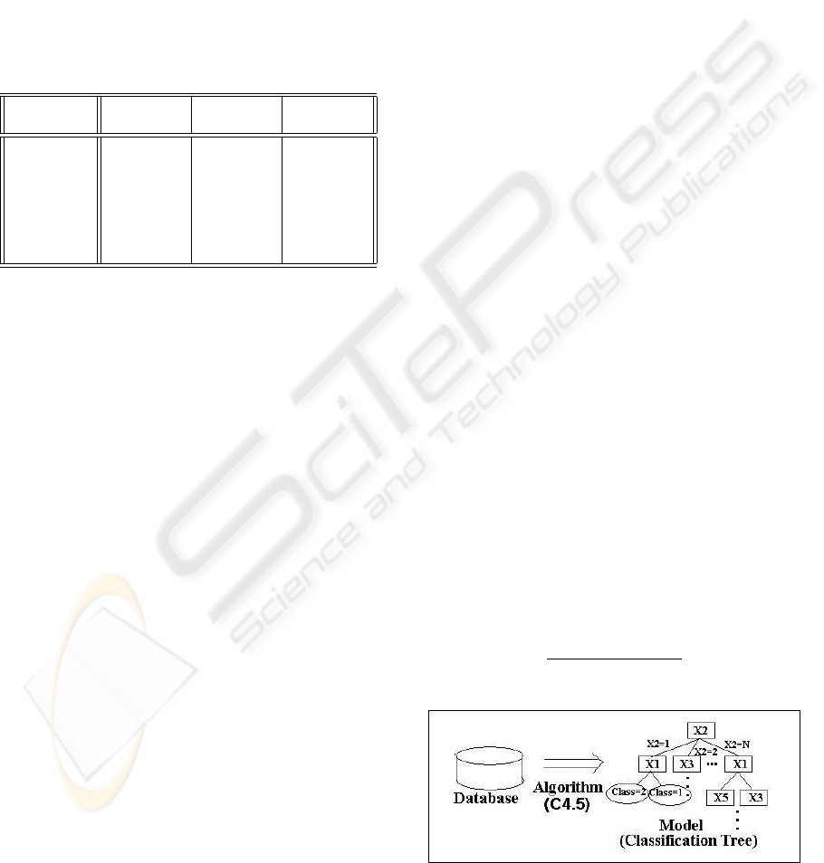
3.2.1 Decision Trees
A decision tree consists of nodes and branches to par-
tition a set of samples into a set of covering decision
rules. In each node, a single test or decision is made
to obtain a partition. The starting node is usually re-
ferred as the root node. In the terminal nodes or leaves
a decision is made on the class assignment.
In each node, the main task is to select an attribute
that makes the best partition between the classes of
the samples in the training set. There are many differ-
ent measures to select the best attribute in a node of
the decision trees. In our experiments, we will use the
well known decision tree induction algorithm C4.5
(Quinlan, 1993). Figure 2 shows the normal use of
this kind of paradigms.
3.2.2 Rule Induction
One of the most expressive and human readable
representations for learned hypothesis are the sets of
IF-THEN rules, where in the IF part, there are con-
junctions and disjunctions of conditions composed
of the predictive attributes of the learning task, and
in the THEN part, the class predicted for the samples
that carry out the IF part appears.
We can interpret a decision tree like the set of rules
generated by a rule induction classifier: the tests
that appear in the way from the root of a decision
tree to a leaf, can be translated to a rule’s IF part,
the predicted class of the leaf also in the THEN
part appears. Some problems that may be overcome
by the rule induction paradigm are: generation of
simple rules when noise is present to avoid the
overfitting and efficient rule generation when using
large databases. In our experiments, we will use
Clark and Nibblet’s (Clark and Nibblet, 1989) cn2
rule induction program.Cn2 has been designed with
the aim of inducing short, simple, comprehensible
rules in domains where problems of poor description
language and/or noise may be present. The rules
are searched in a general-to-specific way, generating
rules that satisfy large number of examples of any
single class, and few or none of other classes. To use
the rule set to classify unseen examples, cn2 applies
a ”strict match” interpretation by which each rule is
tried in order until one is found whose conditions are
satisfied by the attributes of the example to classify.
3.2.3 Naive Bayes And Naive Bayes Tree
Classifiers
Theoretically, Bayes’ rule minimizes error by se-
lecting the class y
j
with the largest posterior prob-
ability for a given example X of the form X =<
X
1
, X
2
, ..., X
n
>, as indicated below:
P (Y = y
j
|X) =
P (Y =y
j
)P (X|Y =y
j
)
P (X)
Figure 2: Typical example of a Machine Learning training
algorithm.
ICEIS 2004 - ARTIFICIAL INTELLIGENCE AND DECISION SUPPORT SYSTEMS
236

Table 2: Details of accuracy level percentages for the
databases.
Inducer C4.5 NB NBTree CN2 Best
Diabetes 72.78 75.66 74.74 73.54 75.66
±05.59 ±04.43 ±03.88 ±05.14
Heart 80.37 83.70 79.26 79.28 83.70
±07.42 ±05.84 ±09.27 ±07.23
Ionosph. 89.75 84.90 89.20 92.32 92.32
±04.67 ±05.57 ±04.51 ±03.03
Monk2 67.14 66.22 64.61 57.67 67.14
±09.37 ±08.86 ±08.19 ±09.16
Pima 73.81 75.90 75.14 73.92 75.90
±05.88 ±05.96 ±05.80 ±26.08
Wine 92.75 97.19 94.94 91.07 97.19
±04.56 ±03.96 ±04.96 ±08.93
Zoo 93.10 87.09 96.09 93.09 96.09
±06.71 ±15.69 ±05.05 ±06.91
Since X is a composition of n discrete values, one
can expand this expression to:
P (Y = y
j
|X
1
= x
1
, ..., X
n
= x
n
) =
P (Y =y
j
)P (X
1
=x
1
,...,X
n
=x
n
|Y =y
j
)
P (X
1
=x
1
,...,X
n
=x
n
)
where P (X
1
= x
1
, ..., X
n
= x
n
|Y = y
j
) is the
conditional probability of the instance X given the
class y
j
. P (Y = y
j
) is the a priori probability that
one will observe class y
j
. P (X) is the prior proba-
bility of observing the instance X. All these param-
eters are estimated from the training set. However,
a direct application of these rules is difficult due to
the lack of sufficient data in the training set to reli-
ably obtain all the conditional probabilities needed by
the model. One simple form of the previous diagnose
model has been studied that assumes independence of
the observations of feature variables X
1
, X
2
, ..., X
n
given the class variable Y , which allows us to use the
next equality
P (X
1
= x
1
, ..., X
n
= x
n
|Y = y
j
) =
Q
n
i=1
P (X
i
= x
i
|Y = y
j
)
where P (X
i
= x
i
|Y = y
j
) is the probability of
an instance of class y
j
having the observed attribute
value x
i
. In the core of this paradigm there is an
assumption of independence between the occurrence
of features values, that is not true in many tasks;
however, it is empirically demonstrated that this
paradigm gives good results in several tasks, typically
in medical domains.
In our experiments, we use this Naive Bayes (NB)
classifier. Furthermore, we use a Naive Bayes Tree
(NBTree) classifier (Kohavi, 1996), which builds a
decision tree applying the Naive Bayes classifier at
the leaves of the tree.
Table 2 shows the accuracy obtained by these clas-
sifiers when applied over the chosen databases.
3.3 Experimental Method
To estimate the accuracy of the classifiers pro-
duced by our algorithm, we performed 10-fold cross-
validation (Stone, 1974). In this validation method,
the data set is partitioned into ten disjoint subsets. In
each fold, one subset is held out as an independent
test set and the remaining instances are used as the
training set. A classification algorithm is then learned
on the training set and tested on the test set.
In the new paradigm presented, a pre-processing is
made on the data. All attribute values are scaled to
the interval [0,1]. Extreme values are squashed by
giving a scaled value of 0 (resp. 1) to any raw value
that is less (resp. greater) than three standard devia-
tions from the mean of that feature computed accross
all instances. We use this approach in order to limit
the efect of outlying values.
3.4 k-NN VS. IPW-k-NN
We have tested our new method against the classical
k-NN. Experiments have been carried out using
three distances: Euclidean, Camberra and Chebychev
(Michalsky et al., 1981). Table 3 shows the mathe-
matical description of each of the used distances.
Table 3: Definition of Euclidean, Camberra and Chebychev
distances.
Euclidean D(x,y) =
p
P
m
i=1
(x
i
− y
i
)
2
Camberra D(x, y) =
P
m
i=1
|x
i
−y
i
|
|x
i
+y
i
|
Chebychev D(x, y) = max
m
i=1
|x
i
− y
i
|
Tables 5, 6 and 7 show performances for each
of this three distances obtained by both k-NN and
IPW-k-NN over the seven databases.
In each table the best performance of k-NN and
IPW-k-NN over the whole range of parametres along
with the value of the parameters for which such per-
formance is achieved (K for k-NN, K
p
, K
c
, α and β
for IPW-k-NN).
The last five rows in the table show the percentage of
ANALYSIS OF THE ITERATED PROBABILISTIC WEIGHTED K NEAREST NEIGHBOR METHOD, A NEW
DISTANCE-BASED ALGORITHM
237

cases (among all the posible combinations of the four
parameters) in which IPW-k-NN performance is sig-
nificantly different from k-NN. We compare k-NN for
a given K with IPW-k-NN for the same value of K
c
.
A Wilcoxon signed rank test (Wilcoxon, 1945) is car-
ried out to check the significance level of differences
between k-NN and IPW-k-NN. We have chosen a
minimum significance level of 95%. The row labeled
equal shows the percentage of cases where differ-
ences are no significatives under this level (95%). The
row labeled better 99, shows the percentage of cases
where IPW-k-NN outperforms k-NN with a signifi-
cance of 99%. The row labeled better 95 shows the
percentage of cases where IPW-k-NN outperforms k-
NN with a significance between 95% and 99%. The
rows labeled worse 99 and worse 95 shows the per-
centage of cases where k-NN outperforms IPW-k-NN
under those significance levels.
As it can be seen, in five out of seven databases,
there are combination of value parameters for which
improvement holds. But, in a blind search through
the range of these parameters, we would have lit-
tle chance to find these values, as they are fewer (in
some cases they are very outnumbered) than values
for which k-NN outperforms IPW-k-NN.
In the next section we show a first approach to try to
characterize the parameter values for which IPW-k-
NN outperforms k-NN.
3.5 Characterization Of Parameter
Values
So far we have shown that IPW-k-NN outperforms
k-NN for several values of K
p
, K
c
, α and β. But this
would be almost useless if we are not able to char-
acterize those values for which such improvement in
performance holds.
To check if such characterization is possible we have
constructed the set consisting of every combination
of values of the four parameters along with the
significance of the performance of the algorithm with
those values over each database. So, the set consists
of 700,000 instances, corresponding to 10 (range
of K
p
) x 10 (range of K
c
) x 100 (range of α) x 10
(range of β) x 7 (number of databases). There is a
different set for each distance (Euclidean, Camberra
and Chebychev), so they are three different sets of
700,000 instances each. An instance is composed
by four features (K
p
, K
c
, α, β) and the variable
corresponding to the class it is associated to. There
are three differents classes: IPW-k-NN outperforms
k-NN with a significance of 95% (class 1), k-NN
outperforms IPW-k-NN with a significance of 95%
(class 2), and there is no significative difference
between k-NN and IPW-k-NN (class 3).
ID3, C4.5 and Naive-Bayes classification algorithms
in MLC++ environment have been tested, in order
to assess the success of all three in the task of
characterizing the values of K
p
, K
c
, α and β, for
which a significative improvement is achieved. The
table shows the number of cases that each algorithm
classifies as belonging to class 1, along with the real
classification of that case. For example, in the first
row we have that for the set of 700,000 instances
corresponding to Euclidean distance, when using ID3
(Quinlan, 1986), a total amount of 8,564 cases are
classified as belonging to class 1. But just 2,096 of
them are really belonging to that class, because the
rest of cases were misclassified, corresponding 2,130
cases to class 2, and 4,338 to class 3.
Table 4: Characterization of K
p
, K
c
, α and β using ID3,
C4.5 and Naive-Bayes.
Distance Classif. class 1 class 2 class 3 Total
ID3 2096 2130 4338 8564
24.47% 24.87% 50.65% 100%
Euclidean C4.5 2322 1502 2265 6089
38.13% 24.67% 37.20% 100%
Naive- 33 10 35 78
Bayes 42.31% 12.82% 44.87% 100%
ID3 535 1842 3067 5444
9.83% 33.83% 56.34% 100%
Camberra C4.5 301 295 284 880
34.21% 33.52% 32.27% 100%
Naive- 0 0 0 0
Bayes − − − −
ID3 977 1135 4191 6303
15.50% 18.01% 66.49% 100%
Chebychev C4.5 0 0 0 0
− − − −
Naive- 0 0 0 0
Bayes − − − −
Analyzing these results we observe that C4.5 al-
gorithm over the set corresponding to Euclidean dis-
tance behaves rather well, with a 38% of cases well
classified, against a 25% whose selection would make
IPW-k-NN perform worse. We consider the rest of
cases (37%) to be neutral, due to the no significance
of the difference of performance over those parame-
ters. From these tables we conclude that Camberra
y Chebychev do not seem to be a good election,
with bad classifications exceeding the number of good
ones.
4 CONCLUSION AND FURTHER
RESEARCH
In this work we have developed and tested a new
distance based algorithm: Iterated Probabilistic
ICEIS 2004 - ARTIFICIAL INTELLIGENCE AND DECISION SUPPORT SYSTEMS
238

Weighted k Nearest Neighbor (IPW-k-NN). Three
distance functions have been used in our experiments:
Euclidean, Camberra and Chebychev.
We have shown that improvements over classic k-NN
are achieved for some values of K
p
, K
c
, α and β, as
well that a characterization of such values is possible
using C4.5 and Euclidean distance.
Further research involves a more straightforward
characterization of the values of parameters for which
improvement holds.
An extension of the presented approach is to select
among the feature subset that better performance
presents regarding to classification. A Feature Subset
Selection (Inza et al., 2000; Sierra et al., 2001)
technique could be applied in order to select which
of the predictor variables should be used. This could
take advantage in the classifier execution process, as
well as in the accuracy. A combination with another
paradigms to improve the accuracy of each of them
(Dietterich, 1997; Lazkano and Sierra, 2003) will
also be experimented.
Experiments with different values of α, corre-
sponding to different levels of neighbourhood β,
might also be another line of research.
ACKNOWLEDGMENTS
This work is supported by the University of the
Basque Country.
REFERENCES
Blake, B. and Mertz, C. (1998). Uci repository of machine
learning databases.
Clark, P. and Nibblet, T. (1989). The cn2 induction algo-
rithm. Machine Learning, 3(4):261–283.
Cover, T. and Hart, P. (1967). Nearest neighbour pattern
classification. IEEE Transactions on Information The-
ory, 13(1):21–27.
Cowell, R. G., Dawid, A. P., Lauritzen, S., and Spiegelhar-
ter, D. J. (1999). Probabilistic Networks and Expert
Systems. Springer.
Dasarathy, B. (1991). Nearest Neighbor (NN) Norms: NN
Pattern Recognition Classification Techniques. IEEE
Computer Society Press.
Dietterich, T. G. (1997). Machine learning research: four
current directions. AI Magazine, 18(4):97–136.
Inza, I., Larra
˜
naga, P., Etxeberria, R., and Sierra, B. (2000).
Feature Subset Selection by Bayesian network-based
optimization. Artificial Intelligence, 123(1-2):157–
184.
Kohavi, R. (1996). Scaling up the accuracy of naive-bayes
classifiers: a decision-tree hybrid. In Proceedings of
the Second International Conference on Knowledge
Discovery and Data Mining, pages 147–149.
Lazkano, E. and Sierra, B. (2003). Bayes-nearest: a new
hybrid classifier combining bayesian network and dis-
tance based algorithms. In Proceedings of the EPIA
2003 Conference. Lecture Notes on Computer Sci-
ence. Springer-Verlag.
Michalsky, R., Stepp, R., and Diday, E. (1981). A Re-
cent Advance in Data Analysis: Clustering Objects
into Classes Characterized by Conjunctive Concepts,
pages 33–56. North-Holland.
Mitchell, T. (1997). Machine Learning. McGraw-Hill.
Quinlan, J. (1986). Induction of decision trees. Machine
Learning, 1(1):81–106.
Quinlan, J. (1993). C4.5: Programs for Machine Learning.
Morgan Kaufmann Publishers, Inc.
Sierra, B. and Larra
˜
naga, P. (1998). Predicting survival
in malignant skin melanoma using bayesian networks
automatically induced by genetic algorithms. an em-
pirical comparision between different approaches. Ar-
tificial Intelligence in Medicine, 14:215–230.
Sierra, B. and Lazkano, E. (2002). Probabilistic-weighted k
nearest neighbor algorithm: a new approach for gene
expression based classification. In KES’2002, Sixth
International Conference on Knowledge-Based Intel-
ligent Information Engineering Systems, pages 932–
939. IOS Press.
Sierra, B., Lazkano, E., Inza, I., Merino, M., Larra
˜
naga,
P., and Quiroga., J. (2001). Prototype Selection and
Feature Subset Selection by Estimation of Distribu-
tion Algorithms. A case Study in the survival of cir-
rhotic patients treated with TIPS. In Proceedings of
the Eighth Artificial Intelligence in Medicine in Eu-
rope. Lecture Notes on Artificial Intelligence, pages
20–29. Springer-Verlag.
Stone, M. (1974). Cross-validation choice and assesment of
statistical predictions. Journal of the Royal Statistic
Society, 36:111–147.
Wilcoxon, F. (1945). Individual comparisons by ranking
methods. Biometrics, 1:80–83.
ANALYSIS OF THE ITERATED PROBABILISTIC WEIGHTED K NEAREST NEIGHBOR METHOD, A NEW
DISTANCE-BASED ALGORITHM
239

Table 5: IPW-k-NN vs. k-NN (Euclidean distance)
Databases Diabetes Heart Ionosphere Monk2 Pima Wine Zoo
k-NN Best 74.16 83.33 85.71 76.51 74.68 95.00 94.00
±04.80 ±07.46 ±04.86 ±05.31 ±05.31 ±04.10 ±10.75
K 9 10 1 5 5 7 1
IPW-k-NN Best 76.75 84.82 86.00 76.74 76.88 95.00 95.00
±04.04 ±07.08 ±04.75 ±05.59 ±05.04 ±04.10 ±09.72
K
p
3 2 1 1 5 1 2
K
c
2 10 1 5 2 7 1
α 0.42 0.01 0.01 0.02 0.72 0.01 0.01
β 2 2 1 10 1 1 1
equal 64.46 85.56 85.25 20.17 64.45 76.37 56.07
better 99% 03.91 08.87 00.88 00.00 06.19 00.00 00.00
better 95% 04.59 04.37 02.25 00.82 05.23 00.00 00.00
worse 99% 19.04 00.03 07.56 62.06 19.42 09.98 33.26
worse 95% 08.00 01.17 04.06 16.95 04.71 13.65 10.67
Table 6: IPW-k-NN vs. k-NN (Camberra distance)
Databases Diabetes Heart Ionosphere Monk2 Pima Wine Zoo
k-NN Best 74.03 84.07 90.57 99.53 72.99 97.22 94.00
±03.35 ±07.21 ±04.27 ±00.98 ±03.76 ±02.93 ±09.66
K 5 10 1 1 5 1 1
IPW-k-NN Best 75.97 84.82 90.57 99.53 75.72 97.22 94.00
±04.91 ±08.45 ±04.27 ±00.98 ±04.86 ±02.93 ±09.66
K
p
3 3 1 1 1 1 1
K
c
6 10 1 1 8 1 1
α 0.33 0.13 0.01 0.01 0.07 0.01 0.01
β 4 9 1 1 10 1 1
equal 63.90 88.13 36.06 16.39 71.20 54.44 69.93
better 99% 05.79 01.36 00.00 00.00 07.67 00.00 00.00
better 95% 12.45 06.60 00.00 00.02 10.37 00.00 00.00
worse 99% 11.75 01.00 50.06 76.94 03.86 36.04 21.17
worse 95% 06.11 02.91 13.88 06.65 06.90 09.52 08.90
Table 7: IPW-k-NN vs. k-NN (Chebychev distance)
Databases Diabetes Heart Ionosphere Monk2 Pima Wine Zoo
k-NN Best 72.99 80.00 85.43 73.49 73.90 92.78 87.00
±04.81 ±11.48 ±05.94 ±06.86 ±04.56 ±06.44 ±08.23
K 10 3 5 2 9 8 1
IPW-k-NN Best 75.58 81.85 88.86 73.49 75.98 92.78 88.00
±05.26 ±09.63 ±05.12 ±06.86 ±05.59 ±07.88 ±07.89
K
p
9 1 5 1 1 1 2
K
c
7 3 1 2 9 3 1
α 0.72 0.51 0.08 0.01 0.37 0.01 0.01
β 1 3 10 1 4 1 1
equal 64.54 76.75 58.18 47.25 61.00 89.29 58.06
better 99% 02.73 00.00 15.48 00.00 06.12 00.00 00.00
better 95% 11.25 00.24 15.34 02.62 08.26 00.01 00.00
worse 99% 14.35 06.09 09.65 36.56 18.79 07.10 37.40
worse 95% 07.13 16.92 01.35 13.57 05.83 04.60 05.54
ICEIS 2004 - ARTIFICIAL INTELLIGENCE AND DECISION SUPPORT SYSTEMS
240