
A DATA WAREHOUSE FOR WEATHER INFORMATION
A Pattern recognition solution for climatic conditions in México
José Torres Jímenez
Computer Science Department, ITESM Morelos,Paseo de la Reforma 182-A, Cuernavaca Morelos, México, CP 62589
Jesús Flores Gómez
Computer Science Department, ITESM Morelos,Paseo de la Reforma 182-A, Cuernavaca Morelos, México, CP 62589
Keywords: Database technologies, Data War
ehouse, Pattern recognition in Data Visualization
Abstract: Data warehouse related technologies, allows to extract, group and analyze historical data in order to identify
information valuable to decision making processes. In this paper the implementation of a weather data
warehouse (WDW) to store Mexico’s weather variables is presented. The weather variables data were
provided by the Mexican Institute for Water Technologies (IMTA), the IMTA does research, development,
adaptation, human resource formation and technology transfer to improve the Mexico’s water management,
and in this way contribute to the sustainable development of Mexico. The implemented WDW contains two
dimension tables (one time dimension table and, one geographical dimension table) and one fact table (that
stores the data values for weather variables). The time dimension table spans over ten years from 1980 to
1990. The geographical dimension table involves many Mexico’s hydrological zones and comes from 5551
measuring stations. The WDW enables (through the dimensions navigation) the identification of weather
patterns that would be useful for: a) agriculture politics definition; b) climatic change research; and c)
contingency plans over weather extreme conditions. Even it is well known, but it is important to mention,
that the data warehouse paradigm (in many cases) is better to derivate knowledge from the data in
comparison to the database paradigm, a fact that was confirmed through the WDW exploitation.
1 INTRODUCTION
In this paper the implementation and use of a
weather data warehouse (WDW) is presented. The
data for constructing WDW was provided by the
Mexican Institute for Water Technologies (IMTA by
its initials in Spanish), the IMTA does research,
development, adaptation, human resource formation
and technology transfer to improve the Mexico’s
water management, and in this way contribute to the
Mexico’s sustainable development.
The motivation to construct WDW comes from
th
e difficulties found to visualize across time and
geographical dimensions in an IMTA’s database
application called SICLIM (the input data for the
data warehouse was taken from this application). It
is expected that the weather data warehouse would
enable the identification of weather trends and
seasonality that could be useful for decision making
processes related to agriculture, contingency plans,
and climatic change research.
The rest of the paper is organized as follows: in
sect
ion 2 the dimensional model for DDW is
explained in detail, in section 3 the schema
integration details are presented, in section 4 the
obtained results are highlighted, and in section 5 the
conclusions derived in the use and implementation
of DDW are presented.
2 DDW DIMENSIONAL MODEL
The first accomplished step for WDW construction
was the study of source data. The source data comes
from the database application SICLIM, the entity-
relationship model of the source database is
presented in Figure 1, the database contains many
catalogue tables (for Mexican political states,
562
Torres Jímenez J. and Flores Gómez J. (2004).
A DATA WAREHOUSE FOR WEATHER INFORMATION - A Pattern recognition solution for climatic conditions in México.
In Proceedings of the Sixth International Conference on Enterprise Information Systems, pages 562-565
DOI: 10.5220/0002616905620565
Copyright
c
SciTePress
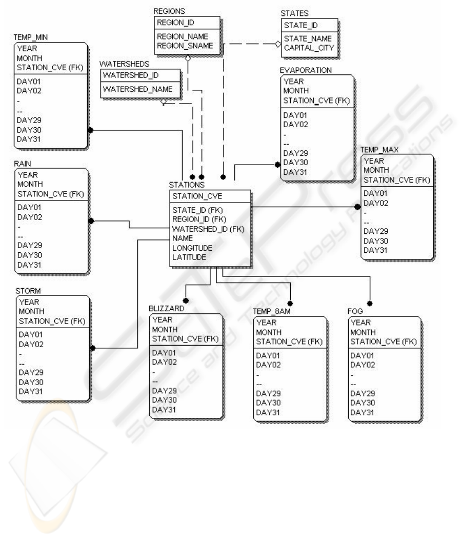
hydrological regions, Watersheds and weather
variable measuring stations).
Figure 1: Relational Model from SICLIM
With this model and the knowledge of IMTA
researches we were able to identify the important
data, as well as the dimensions and hierarchies
required for the dimensional model.
The data identified included the values for rain,
evaporation, maximum temperature, minimum
temperature, temperature at 8 a.m., existence of
storm, blizzard and fog. The cardinality of data, was
daily values. The two dimensions identified where
time, and a hierarchy for the monitoring stations into
regions, watersheds and states.
Time dimension was easy to model, the initial
value of the hierarchy was according to the
cardinality of data, days, and the maximum element
was years. The inside elements include month, two
months period, quarter, four months period ,
semester, and station of the year. The resulting
hierarchy is described on figure 2.
The Station Dimension include the monitoring
station, the state , region and watershed the station
belong . The basic element in the hierarchy was the
monitoring station. However the hierarchy was more
difficult to model than time, since a Region could
extend through several states and a state can hold
several regions. A watershed could also be contained
in several regions inside one state, or through several
A DATA WAREHOUSE FOR WEATHER INFORMATION: A Pattern recognition solution for climatic conditions in
México
563
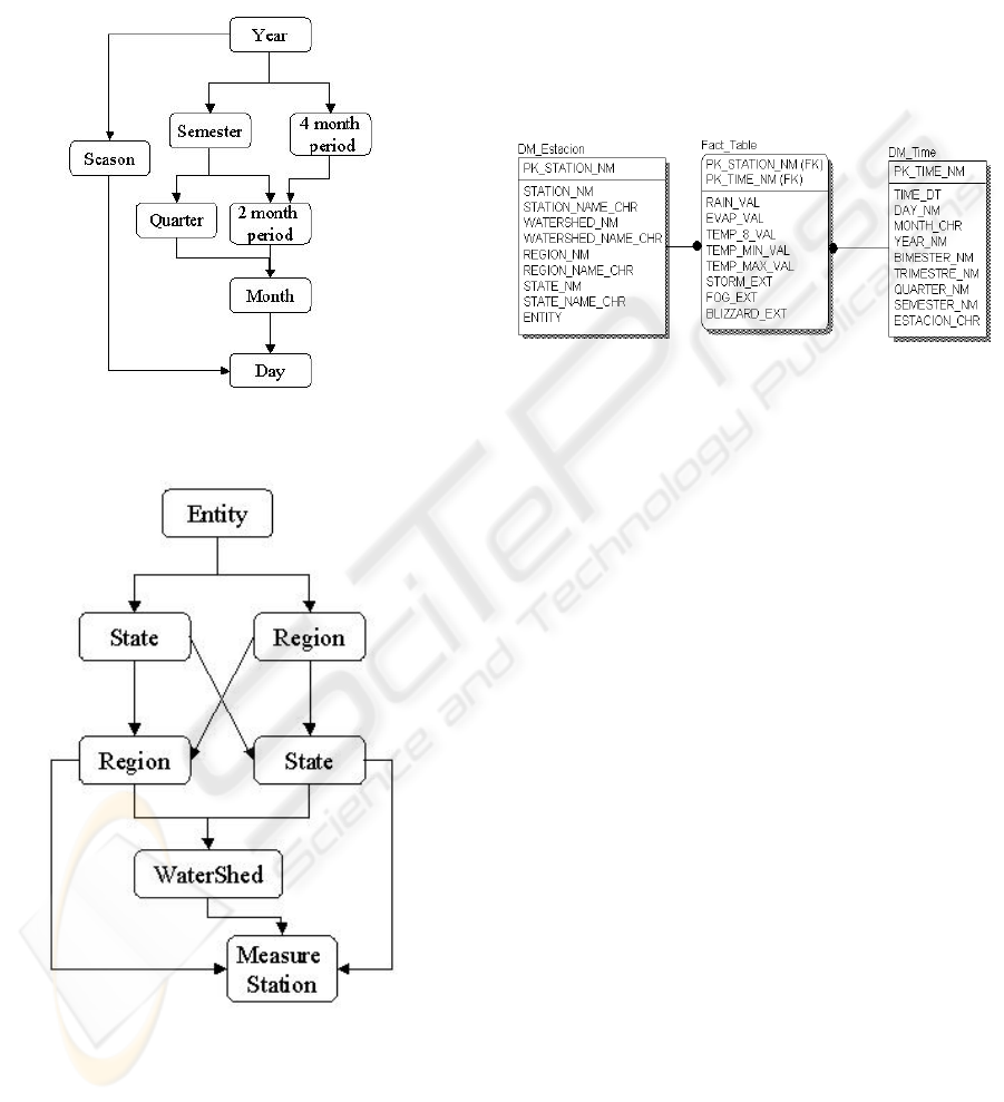
states inside one region. Due to this we needed to
create a new hierarchy element named Entity which
could contain regions and states. Also some stations
didn’t belong to an specific watershed. The final
hierarchy can be observed on figure 3.
Figure 2: Time Hierarchy.
Figure 3: Measure Station Hierarchy
The star diagram of the dimensional model
resulting from this dimensions and data is shown on
Figure 4.
3 SCHEMA INTEGRATION
The next step, was to design the strategy to migrate
the data from the original data source to the data
warehouse. The first step was to decide which
technology use for database purposes. The original
data from SICLIM was contained in Microsoft
Access. The selected technology to store the final
data warehouse was Microsoft SQL Server. The first
step was to import the original data into a database
in the selected Relational database management
system.
Figure 4: Star Diagram for the Data Warehouse
Once migrated, the data contained several null
values and zero values that could be easily identified
as wrong values, for example a day with maximum
temperature of zero with a minimum temperature
above zero. The first step was to identify these
records and generate a strategy to set them with
proper values when possible.
For maximum and 8 a.m. temperature we
checked for missing values or zero values when
minimum temperature was greater then zero, we
looked for neighbour values, and inserted the
average between the two neighbour values. If
neighbour values were missing, we moved to the
next available values, and fill the missing values
with values between the two valid neighbour values.
For minimum temperature, we checked that it was
not greater than maximum value and followed a
similar strategy for wrong or null values. For zero
values we checked for neighbour values, if no value
5 days before of after was 5 or less Celsius degrees
above or below zero, then it didn’t sound possible
for a zero value to be a valid one, and replaced with
an average value of neighbour fields.
For raining and evaporation figure, the missing
values were replaced for average values with
neighbour fields, for zero values, we checked the
previous and next 5 days, if none had a zero value,
then it was modified accordingly to the previous and
following values. Missing values for fog, storm and
blizzard were declared as non existence of the event.
Next we needed to create and load the dimension
tables, for the time dimension we used a program
that automatically inserted a record for each day
between the dates of January 1st, 1980 and
December 31st, 1990. The Dimension key was
ICEIS 2004 - DATABASES AND INFORMATION SYSTEMS INTEGRATION
564

automatically generated using an automated seed
value.
For the monitoring station dimension first we
needed two group regions in two, first group regions
that covered several states, second group regions
present inside the borders of only one state. The
same was to be done with watershed , according to
the region they belonged to, and assign them to the
specific group of its parenting region, or the state
inside its parenting region. Next was to divide the
monitoring stations in groups of those belonging to a
watershed, those not belonging to a watershed but
marked inside a region which would be subdivided
accordingly to the extent of the region across states ,
and finally those not belonging to regions or
watershed and assign them to the state hey were
located. Once it was done we created the entity that
will identify each group, and copied each group into
the monitoring station dimension table. Next step
was to migrate the data from the database to the data
warehouse, however some stations didn’t have
values for all weather variables, even after the zero
and null replacement. One station could have
records for temperature, storm and blizzard, but not
for rain, evaporation and fog. Other station didn’t
have values for complete months of years in any
variable. The missing values would be inserted as
null, marking them not to participate in grouping
operations.
4 RESULTS OBTAINED
The original database occupied around 600 MB in
space, contained in average 726,000 records per
variable table. The data warehouse contained 5,551
records for the monitoring station dimension, 14,975
records for the time dimension and 27,722,823
records in the fact table. The data warehouse
occupied 6,886 MB in space.
Group information was easier to obtain, queries
in SQL where easier to create, and the execution
time was dramatically reduced, for example a query
to obtain the average rain in a region per moth, in
the old database take about 12 minutes, the same
query on the data warehouse only a few seconds.
About the information analysis, through a data
visualization tool we were able to see and identify
some trends in several regions and watersheds. For
example in Lerma-Santiago watershed, the main
raining season occurs from May to September and in
the average temperature at 8 a.m. shows a really
constant curve for a decade.
5 CONCLUSIONS
In this paper a data warehouse to store climatic
Mexico variables was presented. Examples of graphs
evidenced that, using the data warehouse paradigm it
is easier to visualize information (through graphs),
and to navigate over data (using the dimension
hierarchies) in comparison to the traditional database
approach.
One of the big advantages observed in exploiting
the mentioned data warehouse is that complex
grouping queries required using a database
paradigm, reduce to moving through the hierarchies
directed acyclic graphs. In this way the data
warehouse information can be visualized in multiple
ways, enabling the users to identify and to confirm:
a) trends, b) patterns, and c) hypothesis, about
Mexico’s weather variables. The knowledge derived
is a key resource to decision making processes for
every season, watershed, region or state.
The main findings enable the identification of
dominant weather conditions, which could de useful
for planning agricultural strategies according to
climate conditions.
The dimensional model proved to be able to
contain the data warehouse information for a query
intensive application while still being capable of
growth with data from other time periods or
different climatic variables without any major future
development.
REFERENCES
Agrawal, R., Gupta A., Sarawagi S., 1995. Modeling
Multidimensional Databases. In Proc. 13th Int. Conf.
Data Engineering, (ICDE). IEEE Computer Society.
Kimball, R., Reeves L., Ross M., Thornthwaite, W., 1998.
The Data Warehouse Lifecycle Toolkit: expert
methods for designing, developing, and deploying data
warehouses, John Wiley & Sons Inc. USA.
Vassiliadis, P., 1998. Modeling Multidimensional
Databases, Cubes and Cube Operations. In Software
agents activities. In Proc. 10th Int. Conference on
Statistical and Scientific Database Management
(SSDBM).
A DATA WAREHOUSE FOR WEATHER INFORMATION: A Pattern recognition solution for climatic conditions in
México
565
