DYNAMIC DIAGNOSIS OF ACTIVE SYSTEMS WITH

FRAGMENTED OBSERVATIONS

Gianfranco Lamperti

Dipartimento di Elettronica per l’Automazione

Via Branze 38, 25123 Brescia, Italy

Marina Zanella

Dipartimento di Elettronica per l’Automazione

Via Branze 38, 25123 Brescia, Italy

Keywords:

Knowledge-based systems engineering, model-based reasoning, diagnosis, discrete-event systems,

active systems, communicating automata, monitoring, uncertainty

Abstract:

Diagnosis of discrete-event systems (DESs) is a complex and challenging task. Typical application

domains include telecommunication networks, power networks, and digital-hardware networks.

Recent blackouts in northern America and southern Europe oﬀer evidence for the claim that auto-

mated diagnosis of large-scale DESs is a major requirement for the reliability of this sort of critical

systems. The paper is meant as a little step toward this direction. A technique for the dynamic

diagnosis of active systems with uncertain observations is presented. The essential contribution of

the method lies in its ability to cope with uncertainty conditions while monitoring the systems,

by generating diagnostic information at the occurrence of each newly-received fragment of obser-

vation. Uncertainty stems, on the one hand, from the complexity and distribution of the systems,

where noise may aﬀect the communication channels between the system and the control rooms, on

the other, from the multiplicity of such channels, which is bound to relax the absolute temporal

ordering of the observable events generated by the system during operation. The solution of these

diagnostic problems requires nonmonotonic reasoning, where estimates of the system state and the

relevant candidate diagnoses may not survive the occurrence of new observation fragments.

1 INTRODUCTION

Diagnosis is the task of ﬁnding out the faults af-

fecting a physical system given a set of symptoms

gathered by observing the system itself. Model-

based diagnosis is a research area in Artiﬁcial In-

telligence devoted to proposing automated rea-

soning mechanisms and modeling primitives for

performing such a task by exploiting the (struc-

ture and behavior) models of the considered phys-

ical systems. From the middle ’90s some research

eﬀorts have been directed toward model-based di-

agnosis of DESs since discrete models are simpler

to deal with than continuous ones (Fattah and

Provan, 1997; Debouk et al., 2000; Lunze, 2000;

Cordier and Largou¨et, 2001; Pencol´e et al., 2001;

Console et al., 2002) .

Diagnostic processing can be carried out either

after an observation has been collected through-

out a time interval or every time a new observ-

able event is received. In order to distinguish the

two situations we call a posteriori diagnosis the

former task and dynamic (or monitoring-based)

diagnosis the latter.

This paper deals with dynamic diagnosis of ac-

tive systems (Lamperti and Zanella, 2003b). In-

terest on active systems was prompted by the case

study of diagnosis of power transmission networks

(Lamperti and Pogliano, 1997), aimed at prevent-

ing blackouts. Such networks are still a reference

application domain although the notion of an ac-

tive system has progressively been generalized so

as to represent a large class of DESs. The con-

cept of a fragmented observation taken as input

by the task described in this paper is more general

than any one by other authors, corresponding to

an uncertain observation, as deﬁned in (Lamperti

and Zanella, 2002). The only diﬀerence between

an uncertain and a fragmented observation is that

the former cumulatively represents all the observ-

able events received over a time interval while

the latter represents a single (logically uncertain

and/or temporally uncertain and/or source un-

certain) observable event, called a message.

249

Lamperti G. and Zanella M. (2004).

DYNAMIC DIAGNOSIS OF ACTIVE SYSTEMS WITH FRAGMENTED OBSERVATIONS.

In Proceedings of the Sixth International Conference on Enterprise Information Systems, pages 249-261

DOI: 10.5220/0002619202490261

 SciTePress

Past research has focused both on a posteriori

diagnosis (Baroni et al., 1999) and dynamic di-

agnosis (Lamperti and Zanella, 2003a) of active

systems. However, uncertain observations have

so far been provided as input to a posteriori diag-

nosis while dynamic diagnosis had been fed only

by completely certain observations. No contribu-

tion in the literature to monitoring and diagno-

sis of DESs takes into account observable events

that are uncertain in nature. The purpose of the

present work is to face this challenge.

In the remainder of the paper, Section 2

presents the context from which all the examples

in the paper are drawn. Section 3 provides a for-

mal deﬁnition of the class of considered systems.

Section 4 deﬁnes the class of problems inherent

to such systems that can be solved by the tech-

nique described in Section 5. Section 6 relates the

current work to other works in the literature and

concludes the paper.

2 POWER NETWORK

We consider a sample application domain involv-

ing power networks. Each transmission line is

protected by two breakers that are commanded

by a protection. The protection is designed to

detect conditions that may be dangerous to the

line. Typically, if a short circuit aﬀects the line,

the protection is expected to command the two

breakers to open, so as to isolate the line from

the remaining part of the network. In a simpli-

ﬁed view, the network is represented by a series

of lines, each one associated with a protection, as

displayed in Fig. 1.

The ﬁgure outlines a portion of the network,

that encompasses two lines, L

and L

, with rel-

evant protections, p

and p

. For instance, p

controls L

by operating breakers b

and b

. In

normal behavior, both breakers are expected to

open when tripped by the protection. However,

the protection system may exhibit an abnormal

(faulty) behavior, for example, one breaker or

both may not open when required. In such a case,

each faulty breaker informs the protection about

its own misbehavior. Then, the protection sends

a request of recovery actions to the neighboring

protections, which will operate their own break-

ers appropriately. For example, if p

operates b

and b

and the former is faulty, then p

will send

a signal to p

, which is supposed to command

the breaker on the same (left-hand) side of the

faulty breaker b

, namely b

. If both b

and

are faulty, then p

will ask recovery actions

to both the neighboring protections. The protec-

Figure 1: Power network.

tion system is designed to propagate the recovery

request until the tripped breaker opens correctly.

Consequently, the greater the number of faulty

breakers, the larger the extent of the subnetwork

that is isolated.

When the protection system reacts to a short

circuit by attempting to isolate the shorted line,

possibly with the help of recovery actions, a sub-

set of the occurring events are visible to the ex-

ternal world, typically to the operator of a control

room who is in charge of monitoring the behavior

of the network and, possibly, to perform actions

so as to minimize the extent of the isolated sub-

network by means of explicit telecommands. In

the ideal scenario, the reaction of the protection

system is correct (normal) and the shorted line

is clearly identiﬁed by the pair of open breakers.

So, if the operator observes that b

and b

are

open, he or she is allowed to assume that line L

has been isolated owing to a short circuit. If the

short circuit is transient (caused, for example, by

a lightning), it may be the case that, once the

short has extinguished, the isolated line is recon-

nected to the network by the operator. If such a

reconnection is successful (no reaction of the pro-

tection system is triggered anew), the network

keeps on being fully operating. Instead, if the

short circuit is permanent (for example, due to

a tree fallen on the line), the reconnection will

cause a new reaction of the protection system

The reconnection problem becomes harder

when the reaction of the protection system is ab-

normal. In fact, the operator is supposed to face

the additional problem of localizing the shorted

line among those embodied within the isolation.

Such an identiﬁcation cannot be carried out by

simply looking at open breakers. With reference

to Fig. 1, if the open breakers are b

and b

then the shorted line will be either L

or L

. A

static analysis of the isolation does not provide

any clue on where the short circuit is located.

The protection system typically operates au-

tonomously in two steps. First, the shorted line is

isolated for a few seconds in the hope of extinguish-

ing the (transient) short circuit. Later, the line is re-

connected to the network and, if the short circuit has

extinguished, then the network is completely recov-

ered, otherwise the line is isolated permanently from

the system.

ICEIS 2004 - ARTIFICIAL INTELLIGENCE AND DECISION SUPPORT SYSTEMS

250

Assuming the occurrence of a single short cir-

cuit, the only possible claim is that one breaker

is faulty, corresponding to two diﬀerent scenar-

ios. In the ﬁrst scenario, L

is shorted and b

faulty, thereby requiring the intervention of b

The second scenario is symmetric: D

is shorted

and b

is faulty. In either case, one line is not

shorted and might be reconnected without any

risk (provided the operator knows which it is).

For instance, if the shorted line is L

, then L

can be reconnected to the network by opening

manually and telecommanding the closure of

The localization of the short circuit and the

identiﬁcation of the faulty breakers may be im-

practical in real contexts, especially when the ex-

tent of the isolation spans several lines and the op-

erator is required to take recovery actions within

stringent time constraints. On the one hand,

there is the problem of observability: the observ-

able events generated during the reaction of the

protection system are generally incomplete and

uncertain in nature. On the other, whatever the

‘quality’ of the observation, it is practically im-

possible for the operator to reason on the obser-

vations under stringent time constraints, so as to

make consistent hypotheses on the behavior of the

system and, eventually, to establish the shorted

line and the faulty breakers.

The task of the operator might be dramatically

improved if we would provide a tool that supports

the automated reconstruction of the system reac-

tion and the generation of the expected informa-

tion, namely, the diagnosis of the system. This re-

quires the precise deﬁnition of the class of consid-

ered systems, namely active systems, along with a

speciﬁc diagnostic technique. We then show that

our network can be modeled as an active system

and, as such, automatically diagnosed by means

of the given technique.

3 ACTIVE SYSTEMS

A system is a network of components that are

connected to one another through links. Each

component is completely modeled by a commu-

nicating automaton C that reacts to events either

coming from the external world or from neigh-

boring components through links. Formally, the

automaton is a 7-tuple,

C = (S, E

, I, E

out

, O, T, P),

where S is the set of states, E

the set of input

events, I the set of input terminals, E

out

the set

of output events, O the set of output terminals, T

the nondeterministic transition function,

T : S × E

× I × 2

out

×O

7→ 2

and P the priority hierarchy. A transition T ∈ T,

from state S to state S

, that is triggered by

event e at input terminal I, and generates events

, . . . , e

at output terminals O

, . . . , O

, respec-

tively, is denoted by

T = S

(e,I)

−−−−−−−−−−−−→

),...,(e

)

The priority hierarchy is a DAG where nodes are

events in E

×I, while edges denote a partial pri-

ority relationship among events. Since transitions

are triggered by input events, the priority hierar-

chy among events implicitly deﬁnes a priority hi-

erarchy among the transitions in T, speciﬁcally,

if T

has higher priority than T

, T

will be ﬁred

before T

. Generally speaking, among the set of

triggerable transitions, the actual ﬁred transition

will be one among those with highest priority.

Links, which are the means to store the events

exchanged between components, are modeled by

a triple

L = (I, O, M),

where I is the input terminal, O the output ter-

minal, and M the event management. The latter

establishes the internal structure of the link and

the eﬀect of each newly inserted event. Given a

link L, the function Ready(L) returns the set of

(ready) events stored in L that can be consumed

in the current state of the link. For example, if the

event management is a queue, Ready(L) will be

the ﬁrst event in the queue. By contrast, if M is

a stack, Ready(L) will be the last-inserted event.

With a more sophisticated management where

priorities are deﬁned among events stored in L,

Ready(L) is bound to return several consumable

events. The priority hierarchy P of a component

and the event management M of a link L are

diﬀerent, yet related, concepts: the priority re-

lationships in P are applied to those transitions

that are triggered by the events in Ready(L), the

latter depending on M . Since the input terminals

of a component may be connected with a set L

of links, the whole set of consumable events is de-

noted by Ready(L

), corresponding to the union

of the ready events of each link in L

. Formally,

a system Σ is a triple

Σ = (C, L, G),

where C is the set of components, L the set of

links, and G the global priority hierarchy. The

latter is a DAG similar to the priority hierarchy P

of a component model, where the involved events

are pertinent to the whole system rather than to

DYNAMIC DIAGNOSIS OF ACTIVE SYSTEMS WITH FRAGMENTED OBSERVATIONS

251

single components. In other words, G enriches

the DAG obtained by the union of the single P’s

with additional precedence relationships among

the whole set of events in Σ.

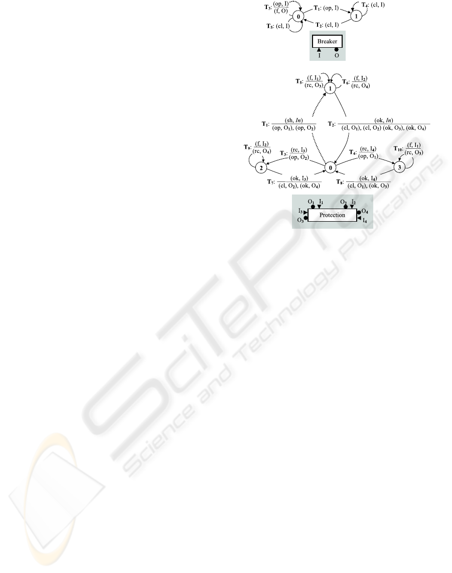
Example 1 Displayed in Fig. 2 are the models

Breaker (top) and Protection (bottom), relevant

to the protection system outlined in Fig. 1. Each

model is depicted by the set of terminals (shaded

box) and the communicating automaton (graph).

Each input terminal is depicted as a triangle,

while each output terminal O is represented as a

bullet. The automaton relevant to the breaker in-

corporates two states, marked by 0 (closed) and 1

(open), respectively, and ﬁve transitions, namely

· · · T

, represented as arrows between states.

When the breaker is closed (state 0), either tran-

sition T

or T

is nondeterministically triggered

by event op on input terminal I. T

moves the

breaker to state 1 (closed) without generating

any output event. T

, instead, keeps the state of

the breaker unchanged (open), whilst generating

event f at output terminal O. Intuitively, this is

an abnormal transition (T

is depicted as a dotted

arrow), as the breaker is supposed to open when

triggered, which is not the case for T

. Event cl

is meant to close the breaker. When in state 1

(open), such an event triggers either T

(normal

behavior) or T

(faulty behavior). Note how the

same event triggers transition T

in state 0, leav-

ing the state unchanged (the breaker was closed

already). No priority relationships are assumed

for the breaker (P is empty).

The model of the protection embodies four in-

put terminals, I

· · · I

, and four output termi-

nals, O

· · · O

. Terminals O

and I

are meant

for connection with the breaker on the left of the

line, while terminals O

and I

are for the com-

munication with the breaker on the right (see

Fig. 1). Instead I

and O

allow the protection

to exchange events with the neighboring protec-

tion on the left. The same applies to I

and O

which are a means to communicate with the adja-

cent protection on the right. The corresponding

automaton involves four states, marked by 0 · · · 3,

and ten transitions, T

· · · T

. State 0 stands for

normal condition. The occurrence of a short cir-

cuit on the protected line is signaled by event sh

from the standard input In, which triggers tran-

sition T

. Such a transition moves the protection

to state 1 by generating event op at both output

terminals O

and O

, thus commanding the two

breakers to open. In state 1, the protection may

receive event f either at terminal I

or I

, mean-

ing that the relevant breaker failed to open. This

triggers either transition T

or T

, respectively,

each of which generates the recovery event rc at

output terminals O

and O

, respectively. The

Figure 2: Component models.

extinction of the short circuit is signaled by event

ok at the standard input terminal In, which trig-

gers transition T

that moves the protection to

state 0, while generating output events cl and ok

at terminals O

and O

, and O

and O

, respec-

tively. When a protection receives a request of re-

covery from a neighboring protection, it follows a

transition from state 0 to either 2 or 3, depending

on whether the request comes from the left (T

) or

from the right (T

), respectively. So, input event

(rc, I

) makes T

to generate (op, O

), that is, a

command to the breaker on the right. In state

2, since even this breaker may in turn be faulty,

the occurrence of event (f, I

) triggers transition

that, similarly to T

, propagates the recovery

request to the right-hand side protection. When

event ok is received at terminal I

from the neigh-

boring protection, transition T

moves the pro-

tection to state 0, while generating cl and ok at

terminals O

and O

, respectively. A symmetric

behavior is deﬁned in state 3. We assume for the

protection a priority hierarchy such that (f, I

)

precedes both (ok, I

) and (ok, In), while both

(rc, I

) and (rc, In) precede (sh, In).

Depicted on the bottom of Fig. 3 is the topol-

ogy of a system Ψ that integrates the three com-

ponents protecting a generic line, namely protec-

tion p and breakers b

and b

. The protection is

connected with the breakers by means of links

· · · L

. We assume that all links share the

same model, where the event management M is

a simple queue. System Ψ is the abstraction of

ICEIS 2004 - ARTIFICIAL INTELLIGENCE AND DECISION SUPPORT SYSTEMS

252

a subpart of the protection system. Larger sub-

parts of the network may be assembled by con-

necting instances of Ψ together by means of links

among protections. The global priority hierar-

chy G of Ψ is such that (cl, I) of both break-

ers precedes (rc, I

), (sh, In), and (rc, I

), while

(op, I) of both breakers precedes (ok, I

), (ok, In),

(ok, I

), (f, I

), and (f, I

). ¤

3.1 Behavior Space

Given an initial state Σ

, system Σ evolves in

a way that is both consistent with its topology

and the behavioral models of its components and

links. The set of all possible evolutions can be

thought of as the behavioral model of Σ starting

at Σ

. The resulting graph is an automaton called

behavior space, Bhv (Σ, Σ

). A (possibly empty)

path between two nodes of the space is a history

segment of Σ. In particular, if the starting node

is the initial state of the space, then such a path

is a history of Σ

Example 2 Shown in Fig. 3 is the behavior

space relevant to system Ψ, where the initial state

is Ψ

= (S

, L

), where S

= (0, 0, 0) and L

in-

volves empty links. In each node, the record S

of the component states for b

, p, and b

is on

the top, while the record L of queues of events

within links L

· · · L

is on the bottom. Inciden-

tally, within the behavior space, at most one event

is stored in each link, so that the state of the

link can be expressed by either the label of the

event or a dash, the latter denoting the empty

link. Labels o and c are a shorthand for op and

cl, respectively. Nodes are marked by numbers

0 · · · 45. For instance, in node 7 both breakers

are closed (state 0 of the breaker model), while

the protection has commanded the breakers to

open (state 1 of the protection model). Besides,

links L

and L

are empty; instead, L

incorpo-

rates event f (meaning that b

has failed to open)

while L

contains event op, meaning that b

has

not yet reacted to the protection command. Each

edge is marked by a label identifying a component

transition. Speciﬁcally, single digits refer to tran-

sitions of the protection, while two-digit strings

correspond to breaker transitions. For example,

3, 31, and 42 stand for T

(p), T

), and T

respectively. Note how Ψ becomes reacting upon

the occurrence of an external event, either from

the standard input (triggering transition T

(p)) or

from a dangling terminal (triggering either T

(p)

or T

(p)).

The behavior space is introduced for formal rea-

sons, but never explicitly generated by the diagnostic

technique.

A history h(Ψ) is identiﬁed by the sequence

of labels (component transitions) marking the

edges on such a path, as for instance, h(Ψ) =

h1, 31, 12, 5i, corresponding to the following sce-

nario: (i) a short circuit occurs on the line pro-

tected by Ψ and protection p commands both

breakers b

and b

to open, (ii) breaker b

fails to

open, while (iii) breaker b

opens correctly, and

(iv) protection p asks the neighboring protection

on the left a recovery action. Finally, note the

cyclicity of Bhv(Ψ, Ψ

), which means that the set

of possible histories of Ψ is unbounded. ¤

4 DIAGNOSTIC PROBLEM

The ultimate task of diagnosis is the solution of

diagnostic problems. Within the domain of active

systems and the context of dynamic diagnosis, a

diagnostic problem concerns the operation of the

system and its solution is essentially based on the

model of the system and some clues on the sys-

tem reaction. Such a solution is a set of candidate

diagnoses, each diagnosis being a set of faults rel-

evant to a possible evolution of the system.

Formally, a fragmented diagnostic problem ℘

for a system Σ is a 4-tuple

℘(Σ) = (Σ

, V, O, R)

where Σ

is the initial state of Σ, that is, the state

of Σ when it starts operating, V is the viewer,

with speciﬁc visibility properties on the behav-

ior of Σ, O is the fragmented observation of Σ

gathered while Σ is operating, and R is the ruler,

which establishes what behavior of Σ is to be con-

sidered faulty and the granularity of the diagno-

sis.

4.1 Viewer

A viewer establishes what component transitions

are somewhat visible, as well as the speciﬁc ob-

servable label for each of them. Let T be the set

of transitions relevant to components in Σ, and V

a set of labels including the null label ε. A viewer

V is a mapping from T to V. If (T, ε) ∈ V, then

T is a silent transition, otherwise T is visible.

Example 3 A viewer V

for Ψ can be deﬁned by

the set of visible transitions

, speciﬁcally V

{(T

(p), sh), (T

(p), l), (T

(p), r), (T

), o

), c

), (T

), o

), (T

), c

)}. ¤

In order to keep the examples within a reasonable

complexity and without loss of generality, we assume

the visibility of the short circuit by means of the sh

label. In real application domains this is of course an

over-assumption.

DYNAMIC DIAGNOSIS OF ACTIVE SYSTEMS WITH FRAGMENTED OBSERVATIONS

253

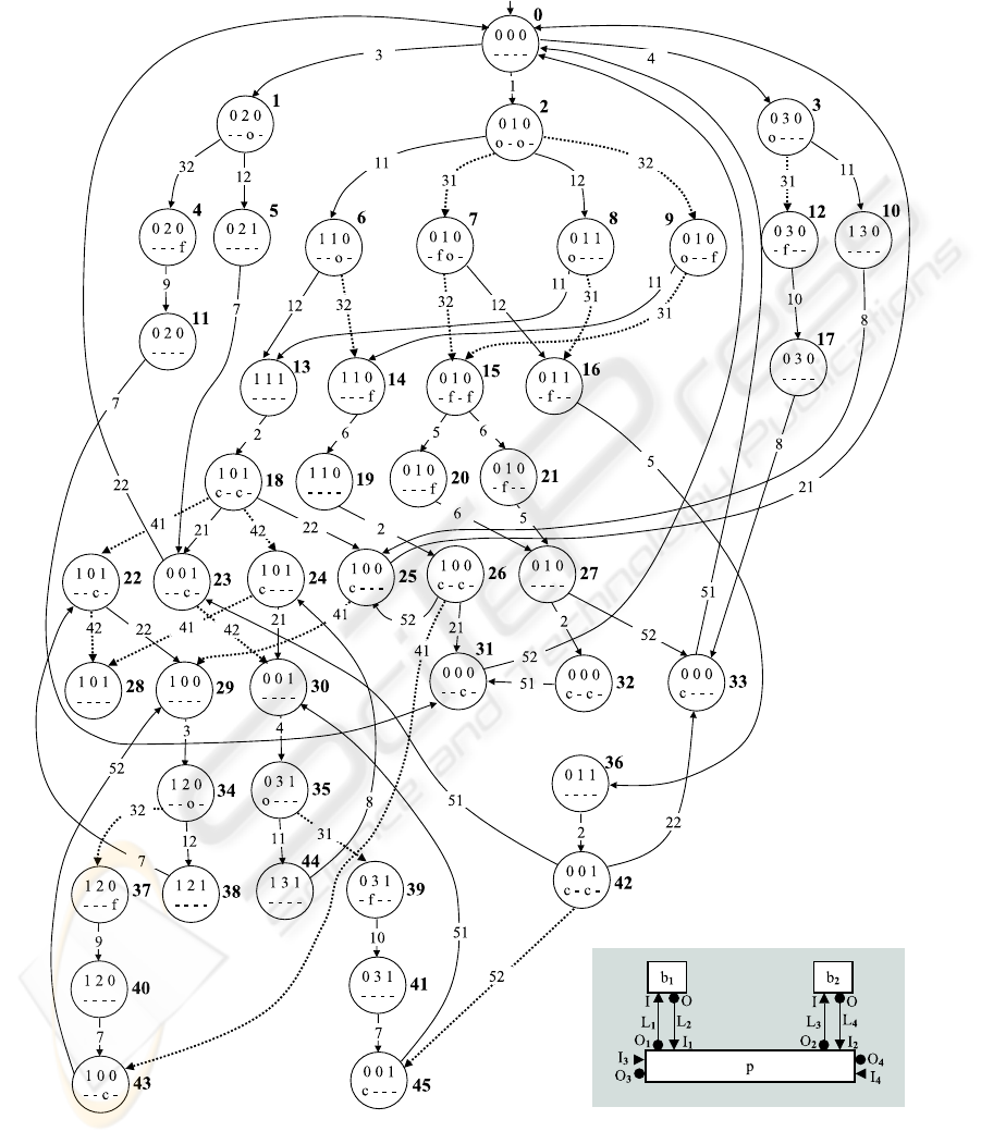
Figure 3: System Ψ (shaded) and behavior space Bhv (Ψ, Ψ

ICEIS 2004 - ARTIFICIAL INTELLIGENCE AND DECISION SUPPORT SYSTEMS

254

4.2 Fragmented Observation

When the system is operating, each visible tran-

sition is perceived by a viewer as a message. Each

message µ is a pair (λ, τ), where λ = {`

, . . . , `

}

is a set of labels in V, namely the logical con-

tent, while τ = {µ

, . . . , µ

} is a set of messages,

namely the temporal content, identifying all the

messages temporally preceding the current one.

A fragmented observation O is a list of mes-

sages,

O = hµ

, . . . , µ

where a monotonicity assumption is assumed:

∀i ∈ [1 .. n], µ

= (λ

, τ

) (τ

⊆ {µ

, . . . , µ

i−1

}).

That is, the temporal content of a message µ is

supposed to refer to a (possibly empty) subset of

the messages preceding µ in O. Thus, a message

is uncertain in nature, both logically and tempo-

rally. Logical uncertainty means that λ includes

the actual (possibly null) label associated with

the transition in V that generated it, but further

spurious labels may be involved too. Temporal

uncertainty means that only partial ordering is

known among messages.

A fragmented observation may be mapped to

an observation graph,

γ(O) = (Ω, Υ, Ω

, Ω

where Ω is the set of nodes isomorphic to the

messages in O, Υ is the set of edges isomorphic

to the temporal contents of messages, Ω

⊆ Ω is

the set of roots, and Ω

is the set of leaves.

A precedence relationship is deﬁned between

nodes of γ(O), speciﬁcally, ω ≺ ω

means that

γ(O) includes a path from ω to ω

, while ω ¹ ω

means either ω ≺ ω

or ω = ω

The graph is supposed to be in canonical form,

that is, if ω 7→ ω

is an edge in Υ, then there does

not exist any ω

such that ω ≺ ω

≺ ω

A sub-observation O

[i]

of O, where i ∈ [0 .. n],

is the (possibly empty) preﬁx of O up to the i-th

message, namely

[i]

= hµ

, . . . , µ

If the following conditions hold:

= ({`

}, ∅), ∀i ∈ [2 .. n] (µ

= ({`

}, {µ

i−1

})) ,

then O is a plain observation, and is denoted by

a list h`

, . . . , `

i of plain messages.

Example 4 A fragmented observation relevant

to viewer V

is O

= hµ

, . . . , µ

i, where µ

({sh}, ∅), µ

= ({o

}, {µ

}), µ

= ({l, ε}, {µ

}),

= ({o

}, {µ

, µ

}), µ

= ({c

}, {µ

}), and

= ({c

, r}, {µ

}). The relevant observation

graph γ(O

) is depicted on the left of Fig. 4. ¤

Figure 4: Observation graph (left) and relevant index

space (right).

4.3 Index Space

Since it is neither trivial nor eﬃcient to reason

about the observation graph as is, an additional

(acyclic) automaton is considered, called the in-

dex space of the observation,

I(O) = (S, E, T, S

, S

where S is the set of states, E = V − {ε} the set

of events, T the transition function, S

the initial

state, and S

the set of ﬁnal states. The pecu-

liarity of an index space lies in that each path

from the root to a ﬁnal node, called a temporal

sequence, represents a mode in which labels may

be chosen in the observation graph without vio-

lating the constraints imposed by temporal and

logical uncertainty. The whole set of such paths

is the extension of I(O), denoted kI(O)k. Note

how each path within the extension is in fact a

plain observation consistent with O.

Example 5 Shown on the right of Fig. 4 is the

index space I(O

). The only ﬁnal state is =

kI(O

)k includes six plain observations. ¤

4.4 Ruler

A ruler establishes what transitions are faulty.

Let T be the set of transitions relevant to com-

ponents in Σ, and R a set of labels including the

null label ε. A ruler R is a mapping from T to

R. If (T, ε) ∈ R, then T is normal, otherwise T is

faulty. A history segment h of Σ is said to imply a

diagnosis δ, where δ is the set of faults associated

with the faulty transitions of h deﬁned in R.

DYNAMIC DIAGNOSIS OF ACTIVE SYSTEMS WITH FRAGMENTED OBSERVATIONS

255

Example 6 A ruler R

for Ψ can be deﬁned

by the set of faulty transitions, namely R

{(T

(p), s), (T

), fo

), (T

), fc

), (T

), fo

, fc

)}. ¤

5 DYNAMIC DIAGNOSIS

During its operation, a system Σ is expected to

react to external events and to generate a collec-

tion of observable events that are received as a

fragmented observation. Based on a fragmented

problem ℘(Σ) = (Σ

, V, O, R), the goal of dy-

namic diagnosis is to compute the set of candi-

date diagnoses at the occurrence of each newly

generated message.

At the beginning, no message is available, that

is, the fragmented observation is empty, namely

O = hi. However, in a strict sense, a ﬁrst set

of candidate diagnoses relevant to the empty ob-

servation should be provided, as Σ might have a

silent reaction involving faulty transitions. At the

occurrence of the ﬁrst message µ

, the monitor-

ing is required to yield the set of candidate diag-

noses relevant to O

[1]

= hµ

i. More generally, if

hµ

, . . . , µ

i is the current sequence of messages,

the occurrence of a new message µ

k+1

causes the

computation of the candidate diagnoses relevant

to O

[k+1]

= hµ

, . . . , µ

, µ

k+1

i. Furthermore, for

each message µ, dynamic diagnosis is required to

compute the set of candidate diagnoses implied by

the occurrence of µ, disregarding the whole set of

candidate diagnoses relevant to the sequence of

messages generated before µ. Thus, at the occur-

rence of the i-th message in O, both such kinds

of candidate sets are to be provided.

5.1 Silent Closure

Ideally, in order to perform dynamic diagnosis, we

need to know the state reached by the system at

the occurrence of each message. However, even in

case the previous state is univocally known, the

current state is bound to be uncertain owing to

silent transitions and the uncertain nature of the

message. On the other hand, the set of possible

states at each newly generated message is con-

ﬁned within a limited domain, this corresponding

to all the states reachable via silent transitions.

This domain is a sort of (silent) closure of the

current state, which encompasses the part of the

behavior space that is transparent to the viewer.

Formally, let σ

be a node of the behavior space

Bhv(Σ, Σ

). The silent closure

Scl(σ

) = (S, E, T, S

, S

out

)

is an automaton such that S

= (σ

, D

) is the

root, and each state S ∈ S is a pair (σ, D) where

σ is a state of Bhv(Σ, Σ

) and D is a set of di-

agnoses δ where σ

Ã σ is a history segment in

Bhv(Σ, Σ

) that implies δ, called the candidate

attribute. E is the set of transitions of Σ.

T : S × E 7→ S is the transition function such

that (σ, D)

−→ (σ

, D

) ∈ T if and only if T is a

silent transition of Σ and σ

−→ σ

is a transition

in Bhv (Σ, Σ

out

⊆ S is the leaving set, deﬁned as follows.

S = (σ, D) ∈ S

out

if and only if there exists a

visible transition σ

−→ σ

in Bhv (Σ, Σ

Example 7 With reference to the behavior

space outlined in Fig. 3, the silent closure of state

5, Scl (5), is the subgraph involving states 5, 23,

and 30, with S

out

= {23, 30}, whose states are

left by visible transitions T

) and T

(p), re-

spectively. ¤

5.2 Monitor

The monitor relevant to a system Σ, an initial

state Σ

, a viewer V, and a ruler R is a graph

Mtr(Σ, Σ

, V, R) = (N, L, E, N

where N is the set of nodes, L the set of labels,

E the set of edges, and N

the initial node. Each

node N ∈ N is an automaton

N = (S, E, T, S

, S

out

) = Scl (S

where S

∈ Bhv(Σ, Σ

). Let

out

[

N∈N

out

(N), S

[

N∈N

(N)},

and V and R the domain of labels in V and R,

respectively. Each edge E ∈ E is marked by a

label in S

out

× (V − {ε}) × R × S

. An edge

(S,`,ϕ,S

)

−−−−−−→ N

where S = (σ, D) and S

= (σ

, D

) are internal

nodes of N and N

, respectively, is such that:

(1) S

= S

), namely, S

is the root of N

;

(2) σ

−→ σ

is a transition in Bhv(Σ, Σ

);

(3) ` is the (visible) label associated with T in V;

(4) ϕ is the label (possibly ε) associated with T in

The initial node N

is such that S

) =

(Σ

, D

Let N be a node of Mtr(Σ, Σ

, V, R). The lo-

cal candidate set ∆

loc

(N) of N is the union of

the candidate attributes relevant to the internal

states of N .

ICEIS 2004 - ARTIFICIAL INTELLIGENCE AND DECISION SUPPORT SYSTEMS

256

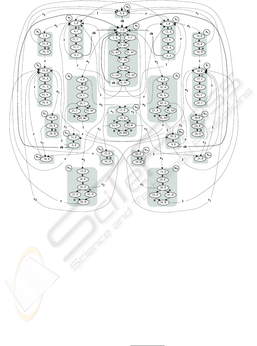
Figure 5: Monitor Mtr(Ψ, Ψ

, V

, R

Example 8 Portrayed in Fig. 5 is an

abstract representation of the monitor

Mtr(Ψ, Ψ

, V

, R

), where V

and R

are

deﬁned in Examples 3 and 6, respectively. Each

node of the monitor is depicted within a shaded

box and labeled by an identiﬁer N

, i ∈ [0 .. 20],

where N

is the root. Within each node, faulty

transitions are marked by letters A, B, C, or D,

which are a shorthand for faults fo

, fc

, fo

and fc

, respectively. Candidate attributes are

written as strings of such letters, e.g., AC is a

shorthand for {{A, C}} = {{fo

, fo

}}. Edges

between nodes are represented as arrows from

the internal state of the leaving node to the root

of the entering node, and marked by the relevant

viewer label. Identiﬁers of component transitions

are omitted (see Fig. 3). ¤

5.3 Monitoring Trajectory

The notion of a monitor allows us to trace the

state of the system based on a given fragmented

observation. However, such a state is uncertain

in nature for three reasons: (i) the uncertain na-

ture of the message, (ii) the unobservability of

the transitions within the nodes of the monitor,

and (iii) the nondeterministic nature of the mon-

itor, where diﬀerent edges leaving the same node

can be marked by the same observable label

Let ℘(Σ) = (Σ

, V, O, R) be a fragmented di-

agnostic problem where O is a plain observation

, . . . , `

i, and Mtr(Σ, Σ

, V, R) = (N, L, E, N

)

a relevant monitor. A context N is a triple

(N, S, H), where N is a node in N, S =

For instance, considering Fig. 5, there are two

diﬀerent edges leaving node N

marked by label c

DYNAMIC DIAGNOSIS OF ACTIVE SYSTEMS WITH FRAGMENTED OBSERVATIONS

257

{δ

, . . . , δ

} is the snapshot context, where each

δ is either an empty set or a singleton incor-

porating the label of a faulty transition, and

H = {δ

, . . . , δ

} is the historic context, where

each δ

is a set of labels relevant to faulty transi-

tions.

The diagnostic join of two sets of diagnoses ∆

and ∆

is a set of diagnoses deﬁned as follows:

∆

on ∆

= {δ | δ = δ

∪ δ

, δ

∈ ∆

, δ

∈ ∆

A monitoring state M is a set {N

, . . . , N

}

of contexts. The monitoring trajectory of ℘(Σ),

Trj (℘(Σ)), is a sequence hM

, M

, . . . , M

i of

monitoring states (inductively) deﬁned as follows:

(1) M

= {(N

, {∅}, {∅)}};

(2) For each i ∈ [1 .. n], M

is the minimal set

of contexts N

= (N

, S

, H

) such that N ∈

i−1

, N = (N, S, H), S ∈ S

out

(N), S =

(σ, D), N

(S,`

,ϕ,S

))

−−−−−−−−−−→ N

∈ E, {ϕ} ∈ S

, and

⊇ (D on H on {{ϕ}})

Example 9 Considering Mtr(Ψ, Ψ

, V

, R

)

displayed in Fig. 5, assume the plain observation

= hsh, o

, li

and the corresponding diagnostic problem

℘

(Ψ) = (Ψ

, V

, O

, R

). The trajectory

Trj (℘

(Ψ)) will be hM

, M

i, where

= {(N

, {∅}, {∅})},

= {(N

, {{s}}, {{s}})},

= {(N

, {∅}, {{s}}), (N

, {∅}, {{s, C}})},

= {(N

, {∅}, {{s, B, C}})}. ¤

5.4 Candidate Sequence

Let ℘(Σ) be a problem involving a plain obser-

vation. A candidate pair

∆ is an association

(∆

, ∆

) of two sets of diagnoses, where ∆

is the

snapshot candidate set, while ∆

is the historic

candidate set.

The candidate sequence

∆(℘(Σ)) is a list

∆

, . . . ,

∆

i deﬁned as follows.

∆

is the

pair (∆

loc

), ∆

loc

)), where N

is the root

of Mtr (Σ, Σ

, V, R), while for each i ∈ [1 .. n],

∆

= (∆

, ∆

), where:

∆

[

(N,S,H)∈M

(∆

loc

(N) on S)

∆

[

(N,S,H)∈M

(∆

loc

(N) on H)

where M

is the monitoring state correspond-

ing to the plain message `

in the trajectory

Trj (℘(Σ)).

By deﬁnition, if ϕ = ε then {ϕ} = ∅.

Example 10 With reference to the diagnostic

problem ℘

(Ψ) deﬁned in Example 9, the candi-

date sequence

∆(℘

(Ψ)) will be h

∆

where

∆

= ({∅}, {∅}),

∆

= ({{s}, {s, A}, {s, C}, {s, A, C}},

{{s}, {s, A}, {s, C}, {s, A, C}}),

∆

= ({∅, {B}, {C}, {B, C}},

{{s}, {s, C}, {s, B, C}}),

∆

= ({∅, {C}}, {{s, B, C}}).

Note how, at the arrival of the third message,

the historic candidate set reduces from the three

candidates of ∆

to the single diagnosis {s, B, C}

of ∆

. ¤

5.5 Index-Space Decoration

The notions of monitoring trajectory and can-

didate sequence have been introduced based on

plain observations. On the other hand, dynamic

diagnosis is meant for solving diagnostic prob-

lems with fragmented observations, where mes-

sages are both logically and temporally uncer-

tain. Such an observation is represented by a

DAG from which an index space can be gener-

ated, as shown in Section 4.3. Each state of the

index space corresponds to several possible ways

in which observable labels may have been gen-

erated by the evolution of Σ, that is, to several

plain observations. Thus, the computation of the

candidate sequence, in the general case, requires

associating each state = of the index space with

the set of monitoring states that are consistent

with all the plain observations relevant to =. In

other words, dynamic diagnosis requires an ex-

tension of the index space.

Let ℘(Σ) = (Σ

, V, O, R) be a fragmented di-

agnostic problem, and I(O) = (S, E, T, S

, S

) the

index space of O. The decoration of I(O) based

on ℘(Σ) is an automaton

∗

(O) = (S

∗

, E

∗

, T

∗

, S

∗

, S

∗

)

isomorphic to I(O), where each state S ∈ S is

marked by a monitoring attribute M as follows:

M =

[

∈kSk

where kSk denotes the set of plain observations

up to S in I(O), O

= h`

, . . . , `

i, ℘

(Σ) =

(Σ

, V, O

, R), Trj (℘

(Σ)) = hM

, M

, . . . , M

Example 11 Consider the diagnostic problem

℘(Ψ) = (Ψ

, V

, O

, R

), where V

, O

, and

ICEIS 2004 - ARTIFICIAL INTELLIGENCE AND DECISION SUPPORT SYSTEMS

258

Table 1: Generation of the diagnostic sequence

∆(℘(Ψ)).

i S

∗

∆

0 {=

} {∅} {∅}

} {{s}, {s, C}, {s, A, C}} {{s}, {s, C}, {s, A, C}}

} {∅, {B}, {C}, {B, C}} {{s}, {s, C}, {s, B, C}}

} {∅, {C}} {{s, B, C}}

} {∅, {B}, {D}, {B, D}} {{s}, {s, B}, {s, D}, {s, B, C}, {s, B, D}, {s, B, C, D}}

} {∅, {B}} {{s}, {s, B}, {s, B, C}}

} {∅} {{s}}

are deﬁned in Examples 3, 4, and 6, respec-

tively. Both the graph and the index space of O

are depicted in Fig. 4. The decoration of I(O) can

be expressed by determining each monitoring at-

tribute M

that is relevant to node =

, i ∈ [0 .. 7],

namely:

= {(N

, {∅}, {∅})},

= {(N

, {{s}}, {{s}})},

= {(N

, {∅}, {{s}}), (N

, {∅}, {{s, C}})},

= {(N

, {∅}, {{s, A, C}})},

= {(N

, {∅}, {{s, B, C}})},

= {(N

, {∅}, {{s}}), (N

, {∅}, {{s, B, C}})},

= {(N

, {∅}, {{s}}), (N

, {∅}, {{s, B}}),

, {∅}, {{s, B, C}})},

= {(N

, {∅}, {{s}})}. ¤

Based on the concept of index-space decoration,

both notions of monitoring trajectory and can-

didate sequence can be straightforwardly gener-

alized to diagnostic problems involving a frag-

mented observation.

Let ℘(Σ) be a problem involving a fragmented

observation O = hµ

, . . . , µ

i. Let I

∗

[i]

) =

∗

, E

∗

, T

∗

, S

∗

, S

∗

) be the decorated index space

relevant to the sub-observation O

[i]

, i ∈ [0 .. n].

The trajectory of ℘(Σ) is the sequence of moni-

toring states hM

, M

, . . . , M

i, where

∀i ∈ [0 .. n]





[

(=,M)∈S

∗





The deﬁnition of the candidate sequence

∆(℘(Σ))

does not change, as M

only depends on the root

of the monitor, while each pair

∆

, i ∈ [1 .. n],

depends upon the monitoring state M

within the

trajectory.

Example 12 With reference to the diagnostic

problem ℘(Ψ) deﬁned in Example 11, the candi-

date sequence

∆(℘(Ψ)) will be h

∆

, . . . ,

∆

as detailed in Table 1. Speciﬁcally, each sub-

observation O

[i]

is associated with the set of ﬁnal

states S

∗

of the decoration =

∗

[i]

), whose mon-

itoring attributes were computed in Example 11.

Note how the historic candidate set reduces to a

singleton {{s}} upon the arrival of the sixth mes-

sage. That is, a short circuit has occurred on the

protected line and the protection apparatus has

reacted correctly. ¤

Algorithm 1 The Diagnose procedure performs

dynamic diagnosis by generating the candidate

sequence relevant to a fragmented diagnostic

problem ℘(Σ) = (Σ

, V, O, R). Each diagnos-

tic pair within the sequence is generated at the

arrival of each message of O. Lines 1–3 create

the roots of the monitor and of the decorated in-

dex space based on the empty observation. The

core of the algorithm is the loop enclosed between

Lines 5–17. Each iteration of the loop is triggered

by the arrival of a new message (Line 6), which

causes the extension of the decorated index space

and of the monitoring space (Lines 7–9). At this

point, possible monitoring states correspond to

the monitoring attributes M of the current ﬁnal

states of the decorated index space. Both snap-

shot and historic candidate sets are computed

based on the contexts incorporated in such at-

tributes M (Lines 12–13), so that the correspond-

ing candidate pair can be eventually generated

(Line 16).

procedure Diagnose(℘(Σ))

input

℘(Σ) = (Σ

, V, O, R): a fragmented problem;

side eﬀects

Incremental generation of Mtr(Σ, Σ

, V, R),

Incremental generation of I

∗

(O ) = (S

∗

, E

∗

, T

∗

, S

∗

, S

∗

Generation of a candidate pair at each new message;

begin

1. Create the root N

of Mtr (Σ, Σ

, V, R);

2. Create the index space of the empty observation;

3. Mark the node of the index space with {(N

, {∅}, {∅)}};

4. Generate (∆

loc

), ∆

loc

));

5. loop

6. µ := the newly received message;

7. Extend the index space based on µ;

8. Extend the monitor based on Step 7;

9. Mark each new state of the index space

DYNAMIC DIAGNOSIS OF ACTIVE SYSTEMS WITH FRAGMENTED OBSERVATIONS

259

with the relevant monitoring attribute M;

10. for each (=, M) ∈ S

∗

11. for each (N, S, H) ∈ M do

12. ∆

:= ∆

∪ (∆

loc

(N) on S);

13. ∆

:= ∆

∪ (∆

loc

(N) on H)

14. end-for

15. end-for;

16. Generate (∆

, ∆

)

17. end-loop

end.

6 CONCLUSION

This paper has introduced a method for comput-

ing diagnoses during monitoring of a class of asyn-

chronous DESs that keep on being called active

systems although they have been endowed with

the new feature of a (local and global) priority hi-

erarchy. Also the notion of a diagnostic problem

has changed, having been introduced both a ruler

and a viewer in its deﬁnition. These new con-

cepts enable to decouple the (behavioral) models

of system components from the descriptions of

their observability and abnormality properties.

In the literature only a more limited separa-

tion between component models and observability

properties can be found: in (Console et al., 2002)

each speciﬁc problem assigns the same observabil-

ity to all the instances of the same component

type whereas each instance can be endowed with

distinct properties in the current approach. It is

worth noting that (Console et al., 2002) gives the

conceptual means to characterize model-based di-

agnosis, not to compute diagnoses, whereas our

proposal encompasses also operational methods.

As to the separation between component models

and abnormality properties, this belongs exclu-

sively to the approach described in the present

paper.

The essential novelty of the paper, however, is

the extension of dynamic diagnosis to fragmented

observations, these being uncertain observations

(Lamperti and Zanella, 2002) such that observ-

able events are received one by one and the re-

ception order does not reﬂect the emission order.

Each received message consists of a logical con-

tent and a (possibly) empty temporal content.

The logical content is uncertain in that it may

range over a set of labels, each of which may have

been emitted by several components. The avail-

able temporal content is uncertain since it does

not allow, in general, to determine one emission

order, instead, it is compliant with several ones.

A limiting monotonicity assumption implicit in

the notion of a fragmented observation is that the

temporal content of each newly received message

cannot place the emission of such a message after

that of any message that has not been received

yet.

The adopted algorithm for dynamic diagnosis

adapts that described in (Lamperti and Zanella,

2003a). However, in (Lamperti and Zanella,

2003a) it was assumed that the label inherent to

each received message was precisely identiﬁed and

the reception order exactly matched the emission

order. In the new algorithm, in order to handle

fragmented observations, the observation index

space is not computed beforehand as in (Lamperti

and Zanella, 2002), instead, it is built incremen-

tally, by updating it every time a new message

is received. This incremental construction, which

directly leads to a deterministic index space with-

out any need of generating a nondeterministic one

ﬁrst, could indeed be proﬁciently exploited also

by a posteriori diagnosis.

The dynamic diagnosis algorithm is inherently

nonmonotonic since, as in (Lamperti and Zanella,

2003a), any estimate of the current system state

may not survive a new message. Orthogonally,

owing to temporal uncertainty in fragmented ob-

servations, every time a new message is received

further sequences of labels may have to be added

to the ones hypothesized so far. However, the

monotonicity assumption prevents any sequence

of labels hypothesized in previous monitoring

steps to be refuted. Future research will tackle

the relaxation of the monotonicity assumption,

thus introducing a second source of nonmono-

tonicity to be coped with by the reasoning mech-

anism. Another plan for future work is to apply

the modeling and reasoning principles described

in this paper to a real-world apparatus.

In the literature, monitoring-based diagnosis

of DESs is considered also by the diagnoser ap-

proach (Sampath et al., 1995; Sampath et al.,

1996) and the incremental decentralized diag-

noser approach (Pencol´e et al., 2001). Both con-

tributions diﬀer from the current method in sev-

eral aspects. First, the class of considered systems

is diﬀerent. In fact, while both the quoted ap-

proaches deal exclusively with synchronous DESs,

the new method can cope with asynchronous

ones, where every system may follow behavioral

silent cycles over time (which is not the case for

the diagnoser approach). Moreover, the exten-

sion of the current method to systems that in-

tegrate synchronous and asynchronous behavior

is straightforward (they are already dealt with in

(Lamperti and Zanella, 2003a), although consid-

ering certain plain observations only). Second,

both approaches consider an observation without

any uncertainty while the method introduced in

this paper takes as input a fragmented observa-

ICEIS 2004 - ARTIFICIAL INTELLIGENCE AND DECISION SUPPORT SYSTEMS

260

tion. Major diﬀerences inherent to the adopted

algorithms are highlighted and discussed in (Lam-

perti and Zanella, 2003a).

REFERENCES

Baroni, P., Lamperti, G., Pogliano, P., and Zanella,

M. (1999). Diagnosis of large active systems.

Artiﬁcial Intelligence, 110(1):135–183.

Console, L., Picardi, C., and Ribaudo, M. (2002).

Process algebras for systems diagnosis. Artiﬁ-

cial Intelligence, 142(1):19–51.

Cordier, M. and Largou¨et, C. (2001). Using model-

checking techniques for diagnosing discrete-

event systems. In Twelfth International Work-

shop on Principles of Diagnosis – DX’01, pages

39–46, San Sicario, I.

Debouk, R., Lafortune, S., and Teneketzis, D. (2000).

A diagnostic protocol for discrete-event systems

with decentralized information. In Eleventh In-

ternational Workshop on Principles of Diagnosis

– DX’00, pages 41–48, Morelia, MX.

Fattah, Y. E. and Provan, G. (1997). Modeling tem-

poral behavior in the model-based diagnosis of

discrete-event systems (a preliminary note). In

Eighth International Workshop on Principles of

Diagnosis – DX’97, Mont St. Michel, F.

Lamperti, G. and Pogliano, P. (1997). Event-based

reasoning for short circuit diagnosis in power

transmission networks. In Fifteenth Interna-

tional Joint Conference on Artiﬁcial Intelligence

– IJCAI’97, pages 446–451, Nagoya, J.

Lamperti, G. and Zanella, M. (2002). Diagnosis of

discrete-event systems from uncertain tempo-

ral observations. Artiﬁcial Intelligence, 137(1–

2):91–163.

Lamperti, G. and Zanella, M. (2003a). Continuous di-

agnosis of discrete-event systems. In Fourteenth

International Workshop on Principles of Diag-

nosis – DX’03, pages 105–111, Washington DC.

Lamperti, G. and Zanella, M. (2003b). Diagnosis

of Active Systems – Principles and Techniques,

volume 741 of The Kluwer International Series

in Engineering and Computer Science. Kluwer

Academic Publisher, Dordrecht, NL.

Lunze, J. (2000). Diagnosis of quantized systems

based on a timed discrete-event model. IEEE

Transactions on Systems, Man, and Cybernetics

– Part A: Systems and Humans, 30(3):322–335.

Pencol´e, Y., Cordier, M., and Roz´e, L. (2001). Incre-

mental decentralized diagnosis approach for the

supervision of a telecommunication network. In

Twelfth International Workshop on Principles of

Diagnosis – DX’01, pages 151–158, San Sicario,

Sampath, M., Sengupta, R., Lafortune, S., Sinnamo-

hideen, K., and Teneketzis, D. (1995). Diagnos-

ability of discrete-event systems. IEEE Trans-

actions on Automatic Control, 40(9):1555–1575.

Sampath, M., Sengupta, R., Lafortune, S., Sinnamo-

hideen, K., and Teneketzis, D. (1996). Fail-

ure diagnosis using discrete-event models. IEEE

Transactions on Control Systems Technology,

4(2):105–124.

DYNAMIC DIAGNOSIS OF ACTIVE SYSTEMS WITH FRAGMENTED OBSERVATIONS

261