AN EFFICIENT FRAMEWORK FOR ITERATIVE TIME-SERIES

TREND MINING

Ajumobi Udechukwu, Ken Barker, Reda Alhajj

ADSA Lab, Dept. of Computer Science, University of Calgary, AB, Canada

Keywords: Trend analysis, Time-series mining, Knowledge discovery and data mining

Abstract: Trend analysis has applications in several domains including: stock market predictions, environmental trend

analysis, sales analysis, etc. Temporal trend analysis is possible when the source data (either business or

scientific) is collected with time stamps, or with time-related ordering. These time stamps (or orderings) are

the core data points for time sequences, as they constitute time series or temporal data. Trends in these time

series, when properly analyzed, lead to an understanding of the general behavior of the series so it is

possible to more thoroughly understand dynamic behaviors found in data. This analysis provides a

foundation for discovering pattern associations within the time series through mining. Furthermore, this

foundation is necessary for the more insightful analysis that can only be achieved by comparing different

time series found in the source data. Previous works on mining temporal trends attempt to efficiently

discover patterns by optimizing discovery processes in a single run over the data. The algorithms generally

rely on user-specified time frames (or time windows) that guide the trend searches. Recent experience with

data mining clearly indicates that the process is inherently iterative, with no guarantees that the best results

are achieved in the first run. If the existing approaches are used for iterative analysis, the same heavy weight

process would be re-run on the data (with varying time windows) in the hope that new discoveries will be

made on subsequent iterations. Unfortunately, this heavy weight re-execution and processing of the data is

expensive. In this work we present a framework in which all the frequent trends in the time series are

computed in a single run (in linear time), thus eliminating expensive re-computations in subsequent

iterations. We also demonstrate that trend associations within the time series or with related time series can

be found.

1 INTRODUCTION

A time series X is an observed data sequence which

is ordered in time, X = x

, t = 1, …, n, where t is an

index of time stamps, and n represents the number of

data observations. Typical examples include stock

market data, weather data, and interaction flow data

(journey to work flows, telephone flows, etc.) A

time series is a sequence of real numbers, and may

be categorical or continuous. Categorical time series

have well defined segments, i.e., portions of the time

series can easily be classified as members of given

categories. For example, given a time series of

precipitation data and the minimum precipitation

that marks a drought. We can easily classify the time

series into periods of drought and periods of normal

precipitation. Translating categorical time series is

thus a trivial problem. However, for continuous time

series there are no well-defined categories. Several

approaches have appeared in the literature for

translating continuous time series: see e.g. (Agrawal

et al., 1995; Faloutsos et al., 1994; Keogh et al.,

2000; Perng et al., 2000; Qu et al., 1998; Yi and

Faloutsos, 2000). Most of the translation schemes

are developed to index and query similar time series.

We are interested in identifying all frequent trends

and trend associations that exist in any given time

series. Trends are qualitative movements that may

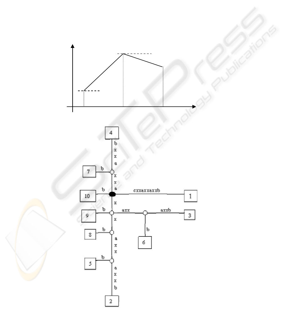
exist in a time series dataset. Figure 1 shows a

repeating trend in a time series. Frequently occurring

trends in time series are excellent pointers for

understanding the general behavior of the series.

130

Udechukwu A., Barker K. and Alhajj R. (2004).

AN EFFICIENT FRAMEWORK FOR ITERATIVE TIME-SERIES TREND MINING.

In Proceedings of the Sixth International Conference on Enterprise Information Systems, pages 130-137

DOI: 10.5220/0002620001300137

 SciTePress

Trends can also be a good start for mining

pattern associations existing within the time series,

or between a time series and other time series. For

example, a sales manager may be interested in

identifying periods when the sales pattern of a

product are similar, or when the sales pattern of a

given product is correlated to the sales patterns of

other products. A major objective of our work is to

achieve such trend discovery in a flexible framework

that allows efficient iterative analysis. Previous work

on time series translation, frequent pattern discovery,

and rule discovery requires domain and application

specific parameters from the users very early in the

process. Hence, the parameters guide (and prejudice)

the entire process. These approaches become

computationally very expensive if the user-specified

parameters and time windows are removed. Our

approach does not require time windows, and can be

applied to any domain. Furthermore, previous works

in the area only address the problem of finding

frequent patterns of a specified length while we lift

this restriction.

The rest of this paper is organized as follows.

Section 2 discusses related work. We discuss our

approach for encoding and finding frequent trends in

Sections 3 and 4. Section 5 discusses our technique

for identifying trend associations. We present the

analysis of our algorithms in Section 6. Our

experimental results are presented in Section 7, and

we conclude in Section 8.

2 RELATED WORK

Time series analysis and mining has received the

attention of several research groups. For example,

Indyk et al (Indyk et al., 2000) study the problem of

identifying representative trends in time series.

Given interval windows, their work aims at

identifying the interval that best approximates (or

represents) its neighbors. The problem they address

is, however, more related to identifying periodic

patterns in time series (Han et al., 1998). Qu et al

(Qu et al., 1998) present an approach for supporting

trend searches in time series data. Their work is in

the general area of time-series query processing and

assumes that the length of the query sequence is

known. The query sequence length is then used as a

window size for processing the time series data. A

match is found if the general trend of the best-fitting

line within a window is the same as that of the query

sequence. Adapting this approach in identifying all

frequent trends will require O(n

) time, thus, it is not

well suited for the problem we address in this paper.

Das et al. (Das et al., 1998) study the problem

of discovering rules in time series. Their approach

uses a sliding window of user-specified width to

extract subsequences from the time series. The

subsequences are then clustered into discrete groups

to complete the translation process. Rules may then

be obtained from the discretized series. Their

approach can be used to find trend associations by

normalizing the data in the subsequences, thus, is

related in spirit to the work presented in this paper.

However, their approach uses user-specified

windows, and would require a quadratic-time, all-

window approach to identify all frequent trends in

the time series. Furthermore, clustering the

subsequences requires the setting of parameters that

is guided by domain knowledge. If no parameters

are set, then, in the worst case, the number of

clusters may approach the number of subsequences

resulting in O(n

) time complexity for an all-window

approach. Other authors have studied rule discovery

in time series from the viewpoint of episodes (Harms

et al., 2001; Mannila et al., 1997). Episodes are

well-defined categories in time series, so they differ

from the problem addressed in this paper.

Patel et al. (Patel et al., 2002) address the

problem of identifying k motifs. A motif, as used in

their work, is a frequently occurring pattern in the

time series. The emphasis of their work is on real

data occurrences and not the movements or trends

existing between data entries. Their algorithm is

based on a user-specified sliding window

(representing the length of the patterns of interest),

and at best runs in sub-quadratic time. Adapting the

algorithm to identify all motifs of arbitrary lengths

will result in O(n

) time complexity, where n is the

size of the time series.

None of the previous works on temporal trend

discovery addresses the problem of finding all

frequent trends of arbitrary lengths. These works are

also guided by user-specified time windows that

dictate the lengths of the trends of interest. As a

Figure 1: An illustration of a repeating trend in time series.

AN EFFICIENT FRAMEWORK FOR ITERATIVE TIME-SERIES TREND MINING

131

result, these previous works generally require O(n

)

time to iteratively discover frequent trends of

arbitrary lengths. Our framework is developed to

support iterative analysis, and discovers all the

frequent trends in linear time.

3 TREND ENCODING

As a first step to time-series trend analysis, the time

series dataset has to be encoded in some way. As

discussed in Section 1, the encoding of categorical

time-series is trivial because the datasets have well

defined segments. Thus, the focus of our discussion

in this section is continuous time series data. The

data range for continuous time series is the set of

real numbers. Hence, as a first step to analyzing

continuous time-series, the data is discretized or

encoded by extracting relevant features from the

series. In our work, we require an encoding scheme

that adequately captures the movements or trends

existing in the time series. We also require an

encoding scheme that does not make use of time

windows so as to maintain efficient support for

iterative analysis. Most time series translation

schemes discussed in the literature require some

form of windows or domain-specific data

categorizations (Das et al., 1998; Faloutsos et al.,

1994; Keogh et al., 2000; Perng et al., 2000; Qu et

al., 1998; Yi and Faloutsos, 2000). Such encoding

schemes are inappropriate for our work.

The work by Agrawal et al. (Agrawal et al.,

1995) encodes the shapes in continuous time series

datasets. Each point in the series is translated based

on the relative change in the value of that point

compared to the previous point. The change can be

captured as a steep increase, increase, steep

decrease, decrease, no-change, or zero. We adapt

and generalize the shape-encoding concept

introduced in (Agrawal et al., 1995) for our work.

Our adapted scheme is discussed below.

3.1 Generalized Trend Encoding

The translation scheme used in this work is simple

and utilizes the relative changes in the time series

values to encode the series into a finite alphabet

string. We utilize a symmetrical alphabet encoding

that allows the matching of reverse patterns. The

underlying thought in our scheme is as follows:

given any two consecutive points on a continuous

time series, and knowing that the time series must be

changing in time; if the time component is

represented on one axis in a two dimensional plane,

then the line joining the two consecutive points must

be less than ninety degrees from the time axis in an

increasing or decreasing direction. Thus, we can

represent the relative movements in the time series

irrespective of the domain from which the data is

drawn. Figure 2 illustrates the overall concept.

The maximum value of angle ab is less than

, as is the maximum value of angle bc. The range

of angular values is maintained irrespective of the

data domain. Movements in the time series are then

simply encoded into alphabets based on the angles

between two neighboring data points. The alphabet

size can be greatly reduced or increased depending

on the level of detail desired. Using fewer alphabets

(i.e., angular categories) will result in approximate

matches.

To complete our discussion on the encoding

scheme, recall that the time component is assigned

to one of the axes. The time component, however, is

not on the same scale as the time series data entries.

The magnitude of the time component affects the

angle between the two data points. A natural choice

for the time unit is the recorded intervals at which

the data elements were collected. Alternatively,

given that the time series data elements were

collected at uniform intervals, and that the focus is

on discovering trends relative to the overall

movements in the series, we can establish a

distributive value for each time unit as follows:

TimeUnit = Change Space / Change Interval

Given a time series X = x

, x

, …, x

;

Change Space =

∑

−

, and

Change Interval = n – 1; where n is the size of the

time series. Given that x

and x

i+1

are two

consecutive entries in the series, and that θ is the

angle between them;

Tan θ =

imeUn

xx ii || 1 −+

The angle of change is then determined, and the

translation for that data point calculated accordingly.

The result is a string of length n-1 where n is the

number of data points in the original time series.

4 IDENTIFYING ALL FREQUENT

TRENDS

This Section presents the main contribution of this

paper, i.e., identifying all the frequent trends in the

time-series in one pass, thus, eliminating expensive

re-computations required by previous works to

achieve iterative analysis. We propose to identify all

frequent trends in any time series dataset by

ICEIS 2004 - ARTIFICIAL INTELLIGENCE AND DECISION SUPPORT SYSTEMS

132

representing the translated time series with a suffix

tree (Bieganski et al., 1994; Gusfield, 1997). Such a

representation would allow the identification of all

frequent trends in linear time. A suffix tree can be

used to represent a string composed from a finite

alphabet. A suffix tree for a string x of length n is a

rooted directed tree with exactly n leaves numbered

1 to n. The internal nodes of the tree, besides the

root node, must have at least two descendants. The

edges are labeled with nonempty sub-strings of x,

and no two edges originating from any particular

node can have edge-labels that start with the same

character. For any leaf i of the tree, the

concatenation of the edge-labels on the path from the

root to leaf i results in the suffix of string x from

position i.

Figure 3 shows the suffix tree for string

“cxxaxxaxxb”. The following nomenclature is used

in the figure: the root node is depicted by a shaded

oval, the internal nodes by unshaded ovals; and the

leaf nodes by rectangles. Each leaf node is the path

taken by a particular suffix of the sequence, and is

named with the start position of that suffix. The label

of each node is the concatenation of all the edge-

labels for the path from the root to that node. The

suffix tree for “cxxaxxaxxb” has five internal nodes

with labels: “x”, “xx”, “xxaxx”, “axx”, and “xaxx”.

The labels of the internal nodes depict repeated parts

of the string. We wish to capture all the meaningful

repeated structures in the series without producing

overwhelming output, so we only select the

maximally repeated patterns that occur in maximal

pairs.

Figure 3: Suffix tree for string “cxxaxxaxxb”.

Time

Figure 2: Relative trends in time series.

AN EFFICIENT FRAMEWORK FOR ITERATIVE TIME-SERIES TREND MINING

133

Definition 1: Maximal pair: A maximal pair (or

maximally repeated pair) in a string s is a pair of

identical substrings r

and r

in s with the property

that the character to the immediate right (left) of r

different from the character to the immediate right

(left) of r

, thus, the equality of the two strings

would be destroyed if r

and r

are extended in either

direction.

Definition 2: Maximal repeat: A maximal repeat m

in string s is a substring of s that occurs in a maximal

pair in s.

Based on the definitions above, only 3 of the 5

node labels in Figure 3 are maximal repeats, these

are: “x”, “xx”, and “xxaxx”. The other repeated

patterns do not have independent occurrences that

are not within the maximal repeats. In our work, all

the patterns that participate in maximal repeats

(including their start and end points) are recorded in

a file using a simple format. The first element of

each record is a unique identifier we assign to each

pattern. The next element is the pattern, then the

number of occurrences of the pattern, and finally the

start and end points of all the occurrences. An

example of such a file is:

0; x; 6; 2,2; 3,3; 5,5; 6,6; 8,8; 9,9

1; xx; 3; 2,3; 5,6; 8,9

2; xxaxx; 2; 2,6; 5,9

Note that we enumerate all the occurrences of the

pattern, and not just its occurrences that are maximal

pairs. Thus, once a pattern has at least one

occurrence as a maximally repeated pattern, we

enumerate all its occurrences. The occurrences of a

pattern begin at all the leaf nodes that descend from

the node that has that pattern as the node label. Note

that both “x” and “xx” have higher occurrence

frequencies and they are sub-patterns of “xxaxx”.

The other repeated patterns always occur within

“xxaxx”, so they do not qualify as maximal patterns,

and can always be generated from “xxaxx”. Our

discussion so far is presented algorithmically below:

Input: Translated sequence (from time series)

Output: File containing maximal repeated

patterns

Steps:

1 Represent sequence with a suffix tree

2 Identify patterns with ≥ 1 maximally

repeated pair. For each pattern identified:

2.1 Assign a unique pattern-ID

2.2 Write the pattern, pattern-ID,

occurrence frequency, and start

and end positions of all its

occurrences to the output file

The steps discussed so far only need to be

carried out once on a given time series dataset. At

this stage, the user can retrieve all patterns of interest

by specifying the minimum frequency of occurrence,

or the minimum length of the pattern, or both. This

operation will require a simple query because we

have already stored all the maximal patterns and

frequencies in a file. This differs from existing

approaches that would require re-computation for

each new query specification.

The discussion so far has used a generalized

notion of repeating patterns. Special sets of repeating

patterns (such as non-overlapping repeats and

tandem repeats) may be derived from the general set

of frequent patterns by comparing the start and end

positions of the repeats.

5 MINING TREND

ASSOCIATIONS

Our algorithm for mining trend associations relies on

the set of maximal patterns found earlier. The

algorithm takes the file containing the set of

maximal patterns as input. The user has to set the

threshold (or minimum allowable) confidence for the

algorithm. For example, given that A and B are two

patterns discovered in the time series; assume

pattern A occurs four times, and that there are three

occurrences where B is found after A. The

confidence of the rule “B follows A” is ¾ (i.e., 75%).

There are also 3 optional user-specified inputs

to the algorithm. The first is the allowable time lag,

with a default of 0. For example, the user may want

the association “B follows A” to mean that B follows

A immediately, or the intent may be that B follows A

within at most 2 time units. The user may also

specify the minimum length of patterns considered

in the trend associations, and (or) the minimum

frequency of occurrence for a pattern to be

considered in the trend associations. These two

parameters aid in pruning the discovered rules to suit

the user’s specific interests. We use a subset of

Allen’s temporal interval logic (Allen, 1983;

Hoppner, 2001) to show the associations that may

exist between patterns in our framework. Figure 4

shows Allen’s interval relationships.

The first three relationships can be realized

between pairs of maximal patterns in our framework.

(The time-lag parameter only applies to the first rule

class.) However, the next three exist within maximal

patterns. For example, given that pattern A is

“xxaxx”, we can generate rules between the subparts

of A, such as “axx” finishes “xxaxx”. Rules like

these are rather obvious once we have the set of

maximal repeats.

ICEIS 2004 - ARTIFICIAL INTELLIGENCE AND DECISION SUPPORT SYSTEMS

134

The first three relationships in Figure 4 give

more interesting mining results. Notice that the

second relationship is equivalent to the first

relationship with zero time lag. To discover these

associations using our framework, we check the start

and end points of each pattern in the set of maximal

repeats against the start/end positions of all other

maximal patterns. For example, given two patterns

with unique id’s 0 and 1, and frequency counts 3 and

2, respectively; as shown below:

0; 3; 1,4; 8,11; 15,18

1; 2; 5,6; 12,13

Assuming a confidence threshold of 0.75, it is easy

to see that the rule “Pattern 0 occurs after Pattern 1

(i.e., every occurrence of pattern 0 follows an

occurrence of pattern 1)” cannot hold because there

are 3 occurrences of pattern 0 and only 2

occurrences of pattern 1, so at best, this rule would

have a 0.67 confidence.

On the other hand, the rule “Pattern 1 occurs

after Pattern 0 (i.e., every occurrence of pattern 1

follows an occurrence of pattern 0)” can be

discovered by comparing the start positions of

pattern 1 with the end positions of pattern 0. In

general, given that X.start represents the start point

of pattern X, and X.end represents the end point of

pattern X. Rules of the form “Pattern A occurs after

Pattern B (i.e., every occurrence of pattern A follows

an occurrence of pattern B)”, can be discovered by

finding the percentage of the occurrences of pattern

A that satisfy the inequality 0

≤ A.start – B.end ≤

time lag. This percentage must be up to the threshold

confidence for the rule to be returned (as true) to the

user. Similarly, rules of the form “Pattern A occurs

before Pattern B (i.e., every occurrence of pattern A

precedes an occurrence of pattern B)”, can be

discovered by finding the percentage of the

occurrences of pattern A that satisfy the inequality

≤ B.start – A.end ≤ time lag. The overlapping

relationship can be similarly defined.

Our framework can also be used to identify

associations between trends/patterns in multiple time

series. Each time series is encoded into a string, and

the maximal repeat patterns are extracted and stored

in a file using the techniques discussed earlier. The

rules are mined in the same way as those for a single

time-series, however, we can now define inequalities

to extract relationships in the form of the last four

Allen’s rules (see in Figure 4).

6 ANALYSIS

Our framework is composed of the following steps:

Step 1: Translation: Given that the time series has N

data elements, the translation takes O(N) time. The

result is a string of length N-1.

Step 2: Retrieving all frequent patterns: The suffix

tree is built in O(N) time. The disk-based approach

to suffix tree construction also runs in O(N) time.

Identifying the maximal repeats from the suffix tree

takes O(N) time. Thus, all the maximal frequent

patterns in our framework can be retrieved in linear

time.

Step 3: Mining trend associations: The time

required to discover the trend associations depends

on the number of maximal patterns, n. Each pattern

is compared with every other pattern in the file, thus

the operation runs in O(n

) time. In the worst case (if

the entire sequence is made up of the same

character), n = N-1. The number of participating

patterns may also be reduced by user-specified

parameters (such as minimum pattern-length and/or

time

A after B B before A

A is-met-by B B meets A

A is-overlapped-by B B overlaps A

A finishes B B is-finished-by A

A during B B contains A

A is-started-by B B starts A

A equals B B equals A

Figure 4: Allen’s interval relationships (Hoppner, 2001)

AN EFFICIENT FRAMEWORK FOR ITERATIVE TIME-SERIES TREND MINING

135

frequency). For practical applications, however, the

time series would be encoded with more than one

character, and patterns spanning multiple time

periods (e.g., ≥ 4) would be of greater interest, thus n

<< N.

7 EXPERIMENTAL EVALUATION

In our experiments we make use of several publicly

available datasets (Keogh, 2003; West, 2003). We

begin by translating each time series dataset. We

define 52 angular categories for encoding the

movements between pairs of entries in the time

series. Twenty-six of the categories are used for

increasing trends while the other twenty-six encode

decreasing trends. We use the average change space

to represent the time axis (see the discussion in

Section 3.1). The angular categories for increasing

movements are as follows: 0 – 39 degrees are

encoded with the letters a – h respectively, with 5-

degree increments between categories; 40 – 49

degrees are encoded with letters i – r respectively,

with 1-degree increments; 50 – 90 degrees are

encoded with letters s – z respectively, with 5-degree

increments. Decreasing trends are encoded in capital

letters using the same categories. We use more

discriminatory categories for angular changes

between 40 and 49 degrees. This is because the

mean movement has an angular change of 45

degrees when the time axis is represented by the

mean change space. Table 1 gives a summary of our

results on different datasets using 52 angular

categories. Reducing the number of categories used

can discover more approximate patterns. Table 2

shows the summary of our results when the angular

categories are reduced to 3. For both experiments,

time lag is set to 10 periods and threshold

confidence is 0.80. (Time-lag and confidence are

used for identifying trend associations. See the

discussion in Section 5). For the second experiment,

angular changes between –10 and +10 are taken as

no change (n), changes greater than 10 degrees are

encoded as increasing or decreasing trends (i or d)

respectively, depending on the direction of change.

Notice that for both experiments, the number of

frequent patterns is much smaller than the number of

entries in the time series. The number drops further

if the minimum pattern length is set ≥ 4. Notice also

that more frequent trends are reported in Table 2 for

each of the datasets. The trends are also longer and

generally occur more frequently. There are also

more trend associations. The increases are due to the

approximate matching achieved by using fewer

angular categories. The number of categories to use

should be guided by the analysis task at hand.

Generally, broader categories may be used to

identify broad segments of the time series with

similar movements. More discriminatory categories

however, should be used if identifying interesting

trend associations is the objective.

8 CONCLUSIONS

In this paper we have addressed the problem of

identifying all frequently occurring trends in time

series. We also show how to identify associations

existing in the discovered frequent trends. A major

underlying theme of the work presented in this paper

is the support for iterative trend discovery and

mining. The mining framework used in this paper is

well suited for both categorical and continuous time-

series datasets. Existing approaches for time series

trend discovery and mining require domain-specific

input very early in their processes, thus, the domain-

specific variables (such as time windows) drive the

subsequent stages of these algorithms. Our approach

does not make use of time windows, thus, all the

frequent trends existing in the dataset are identified

in the first pass. The identified trends are stored and

simply queried for subsequent analysis. Hence, our

approach is better suited for iterative trend analysis

because it does not require expensive re-computation

when parameters are changed during analysis.

Table 1: Summary of results with 52 angular categories

Dataset Length Number of

frequent

trends

Frequent trends

spanning at ≥ 4

time periods

Average freq. of

trends spanning

≥ 4 periods

Num. of trend

associations

Balloon 2001 768 412 5 31

Darwin 1400 421 1 2 5

Foetal_ecg 2500 694 22 2 10

Greatlakes 984 328 3 2 15

Industrial 564 190 1 2 17

Soiltemp 2304 772 90 2 20

Sunspot 2899 841 32 6 9

ICEIS 2004 - ARTIFICIAL INTELLIGENCE AND DECISION SUPPORT SYSTEMS

136

Table 2: Summary of results with 3 angular categories

Dataset Length Number of

frequent

trends

Frequent trends

spanning at ≥ 4

time periods

Average freq. of

trends spanning

≥ 4 periods

Num. of trend

associations

Balloon 2001 1200 1161 6 101

Darwin 1400 743 705 9 330

Foetal_ecg 2500 1510 1471 6 159

Greatlakes 984 510 471 8 221

Industrial 564 346 316 7 114

Soiltemp 2304 1404 1365 7 176

Sunspot 2899 1783 1744 7 159

REFERENCES

Agrawal, R., Psaila, G., Wimmers, E.L., and Zait, M.,

1995. Querying Shapes of Histories, Proceedings of

the 21

VLDB Conference, Zurich, Switzerland.

Allen, J.F., 1983. Maintaining Knowledge about Temporal

Intervals, Comm. ACM, 26(11):832-843.

Bieganski, P., Riedl, J., Carlis, J.V., and Retzel, E.R.,

1994. Generalized Suffix Trees for Biological

Sequence Data: Applications and Implementation, In

Proceedings of the 27

Hawaii Int’l Conference on

Systems Science, IEEE Computer Society Press, pages

35-44.

Das, G., Lin, K-I., Mannila, H., Ranganathan, G., and

Smyth, P., 1998. Rule Discovery from Time Series,

Proceedings of the 4

International Conference on

Knowledge Discovery and Data Mining, [KDD98],

New York, NY, pages 16-22.

Faloutsos, C., Ranganathan, M., and Manolopoulos, Y.,

1994. Fast Subsequence Matching in Time-Series

Databases, in Proceedings of the 1994 ACM SIGMOD

International Conference on Management of Data,

pages 419-429.

Gusfield, D., 1997. Algorithms on Strings, Trees, and

Sequences: Computer Science and Computational

Biology, Cambridge University Press.

Han, J., Gong, W., and Yin, Y., 1998. Mining Segment-

Wise Periodic Patterns in Time Series Databases,

KDD, pages 214-218.

Harms, S.K., Deogun, J., Saquer, J., and Tadesse, T.,

2001. Discovering Representative Episodal

Association Rules from Event Sequences Using

Frequent Closed Episode Sets and Event Constraints,

Proceedings of the IEEE International Conference on

Data Mining, Silicon Valley, CA, pages 603-606.

Hoppner, F., 2001. Discovery of Temporal Patterns,

Learning Rules about the Qualitative Behaviour of

Time Series, in De Raedt, L., Siebes, A., (Eds.),

PKDD 2001, LNAI 2168, Springer-Verlag, Berlin,

pages 192-203.

Indyk, P., Koudas, N., and Muthukrishnan, S., 2000.

Identifying Representative Trends in Massive Time

Series Data Sets Using Sketches, In Proceedings of the

Int’l Conference on Very Large Data Bases,

Cairo, Egypt, pages 363-372.

Keogh, E., 2003. The UCR Time Series Data Mining

Archive,

http://www.cs.ucr.edu/~eamonn/TSDMA/index.html

University of California – Computer Science and

Engineering Department, Riverside, CA.

Keogh, E.J., Chakrabarti, K., Pazzani, M.J., and Mehrotra,

S., 2000. Dimensionality Reduction for Fast Similarity

Search in Large Time Series Databases, Journal of

Knowledge and Information Systems, vol 3, number 3,

pages 263-286.

Mannila, H., Toivonen, H., and Verkamo, A.I., 1997.

Discovery of Frequent Episodes in Event Sequences,

Report C-1997-15, Department of Computer Science,

University of Helsinki, Finland.

Patel, P., Keogh, E., Lin, J., and Lonardi, S., 2002. Mining

Motifs in Massive Time Series Databases, Proceedings

of the IEEE Int’l Conference on Data Mining,

Maebashi City, Japan.

Perng, C-S., Wang, H., Zhang, S.R., and Parker, D.S.,

2000. Landmarks: A New Model for Similarity-,

Based Pattern Querying in Time Series Databases,

Proceedings of the 16

IEEE International Conference

on Data Engineering.

Qu, Y., Wang, C., Wang, X.S., 1998. Supporting Fast

Search in Time Series for Movement Patterns in

Multiple Scales, Proceedings of the ACM 7

International Conference on Information Management,

pages 251-258.

West, M., 2003. Some Time Series Data Sets, retrieved

June 18, 2003, from

http://www.stat.duke.edu/~mw/ts_data_sets.html

Duke University.

Yi, B-K, Faloutsos, C., 2000. Fast Time Sequence

Indexing for Arbitrary L

norms, in The VLDB

Journal, pages 385-394.

AN EFFICIENT FRAMEWORK FOR ITERATIVE TIME-SERIES TREND MINING

137