HIERARCHICAL MODEL-BASED CLUSTERING FOR

RELATIONAL DATA

Jianzhong Chen, Mary Shapcott, Sally McClean, Kenny Adamson

School of Computing and Mathematics, Faculty of Engineering, University of Ulster

Shore Road, Newtownabbey, Co. Antrim, BT37 0QB, Northern Ireland, UK

Keywords:

Hierarchical model-based clustering, relational data, frequency aggregates, EM algorithm.

Abstract:

Relational data mining deals with datasets containing multiple types of objects and relationships that are pre-

sented in relational formats, e.g. relational databases that have multiple tables. This paper proposes a proposi-

tional hierarchical model-based method for clustering relational data. We ﬁrst deﬁne an object-relational star

schema to model composite objects, and present a method of ﬂattening composite objects into aggregate ob-

jects by introducing a new type of aggregates – frequency aggregate, which can be used to record not only the

observed values but also the distribution of the values of an attribute. A hierarchical agglomerative clustering

algorithm with log-likelihood distance is then applied to cluster the aggregated data tentatively. After stopping

at a coarse estimate of the number of clusters, a mixture model-based method with the EM algorithm is devel-

oped to perform a further relocation clustering, in which Bayes Information Criterion is used to determine the

optimal number of clusters. Finally we evaluate our approach on a real-world dataset.

1 INTRODUCTION

Clustering aims at determining the intrinsic structure

of clustered data when no information other than the

observed values is available. Three types of clustering

methods have been widely used – hierarchical clus-

tering (Meil

a and Heckerman, 1998), partition-based

clustering and model-based approach using mixture

models (Fraley and Raftery, 1998).

Most traditional clustering methods handle datasets

that have single relation in ﬂat formats. Recently,

there has been a growing interest in relational data

mining (RDM) (D

zeroski and Raedt, 2003; D

zeroski

and Lavra

c, 2001), which is tackling the problem of

mining relational datasets that contain multiple types

of objects and richer relationships and are presented

in relational formats that have more than one ta-

ble. RDM provides techniques for discovering use-

ful or unknown patterns and dependencies embed-

ded in relational databases. A common solution to

RDM is developing propositional methods that in-

tegrate traditional data mining techniques into rela-

tional data by converting or “ﬂattening” multiple ta-

bles into a single table on which standard algorithms

can be run. One of the shortcomings of this approach

is that it may cause loss of meaning or information.

Another solution leads to relational approaches that

are capable of dealing with data stored in multiple

tables directly in the areas of inductive logic pro-

gramming (ILP) (D

zeroski and Raedt, 2003; D

zeroski

and Lavra

c, 2001) and probabilistic relational models

(PRMs) (Friedman et al., 1999). Some initial work of

relational data classiﬁcation and clustering based on

ILP and PRMs have been developed in (D

zeroski and

Raedt, 2003; D

zeroski and Lavra

c, 2001; Emde and

Wettschereck, 1996; Taskar et al., 2001).

In this paper, we present a propositional method

which integrates traditional hierarchical model-based

clustering algorithms with relational data that is com-

posed of a set of composite objects. We use aggrega-

tion to efﬁciently ﬂatten composite objects into ﬂat

aggregate objects, to which model-based hierarchi-

cal agglomerative clustering with log-likelihood dis-

tance and the EM algorithm are then applied. In order

to discover rich aggregate knowledge from relational

data, we deﬁne frequency aggregates for composite

objects, which have vector data type and can be used

to record not only the observed values but also the dis-

tribution of the values of an attribute. Frequency ag-

gregates provide extended semantics in reducing the

information loss during aggregation and are helpful to

the computation of log-likelihood distance.

Chen J., Shapcott M., McClean S. and Adamson K. (2004).

HIERARCHICAL MODEL-BASED CLUSTERING FOR RELATIONAL DATA.

In Proceedings of the Sixth International Conference on Enterprise Information Systems, pages 92-97

DOI: 10.5220/0002624300920097

 SciTePress

2 OBJECT-RELATIONAL STAR

SCHEMA

Multi-relational data mining focuses on composite

objects. A general characterization deﬁnes a compos-

ite object consisting of several components (possibly

from different types) with relationships in between.

We assume the relationship between a composite ob-

ject and its components is aggregation and the objects

are stored in multiple database tables. A composite

object is deﬁned as composed of a base (sub-object)

associated with a set of additional parts (sub-objects).

Two types of composite objects are distinguished cor-

responding with the two kinds of aggregation deﬁned

in object-oriented modelling – shared aggregation,

where the parts may be parts in any wholes, and com-

position aggregation, in which the particular parts are

owned by one whole at a time and the existence of

the parts is strongly dependent on the existence of the

whole (Eriksson and Penker, 1998).

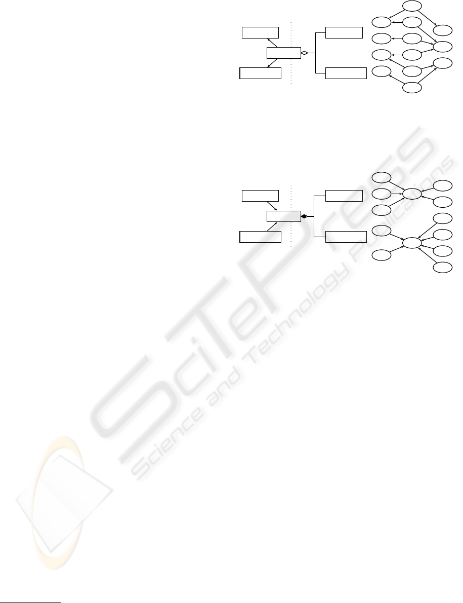
Two types of relational models can be used to

represent the two kinds of aggregation relationships

between the tables. One is relational star schema

(which can be generalized to the relational snowﬂake

schema), where the base table is in the middle and

the part tables radiate from the base

. A relational

star schema represents a shared aggregation in the

way that many-to-one relationships are speciﬁed from

base to parts. In comparison, a so called relational

aggregate schema, where in the middle is the base ta-

ble and the parts converge on the base, is deﬁned to

represent a composition aggregation in the way that

many-to-one relationships are denoted from parts to

base. Figures 1 and 2 illustrate the schema graphs

and object diagrams of the two schemas respectively.

For example, it is natural to design a product sales

database using a relational star schema (Figure 1),

in which each sale is a composite object with a base

object of SaleRecord class (X

) and several sharable

part objects of classes ({X

}) such as Product, Time,

Geography, etc. An example of a relational aggre-

gate schema (Figure 2) used in the paper is to model

a housing condition survey database as composed of

a base table of Dwelling and two part tables of Occu-

pants and Rooms. In this way, each house is repre-

sented as a composite object that has a dwelling de-

scription record, a set of occupants who are living in

and a set of rooms of different living conditions.

The two schemas can be uniﬁed in the object-

relational (OR) context by introducing object iden-

tiﬁers (OIDs), reference (REF) and collection data

types (nested tables or collection of REF types) (Con-

nolly and Begg, 2002), which allow us to convert

The star schema is widely used in data warehousing

and OLAP, where the base table and part tables are called

the fact table and dimension tables respectively.

: base

: part

· · · · · ·

: part

· · · · · ·

: part

∗

(a)

(b)

Figure 1: (a)The schema graph of relational star schema.

(b)An instance graph of relational star schema, including

6 composite objects, that contain 6 objects of base class X

4 objects of part class X

and 3 objects of part class X

: base

: part

· · · · · ·

: part

· · · · · ·

: part

∗

(a)

(b)

Figure 2: (a)The schema graph of relational aggregate

schema. (b)An instance graph of relational aggregate

schema, including 2 composite objects, that contain 2 ob-

jects of base class X

, 5 objects of part class X

and 6 ob-

jects of part class X

the many-to-one relationship in a relational aggregate

schema from parts-to-base into base-to-parts. In this

way, a relational aggregate schema can be replaced by

a star schema. We call the resulting schema as object-

relational star schema which is treated as a uniﬁed

representation of the relational star schema and rela-

tional aggregate schema. For the sake of simplicity,

we assume that only one composite class exists in the

dataset without recursive structures.

More formally, an object-relational star schema de-

ﬁnes a composite class X = {X

, X

, . . . , X

which consists of a base class X

and a set of

part classes {X

, . . . , X

}. Each class X

, 0 ≤

k ≤ K, is an abstract type of an entity in the

domain, and is associated with a set of attributes.

For a star schema, the base class is denoted as

(o, A

, . . . , A

, R

, . . . , R

) and the k-th part

class as X

(o, A

, . . . , A

). Three types of at-

tributes are distinguished. X

.o is used to specify an

unique system-generated object identiﬁer for each ob-

ject of class X

. A descriptive attribute X

, 1 ≤

m ≤ M

, represents an attribute of X

and takes

value from its domain Dom(X

). A reference

attribute X

, 1 ≤ k ≤ K, has domain of REF

HIERARCHICAL MODEL-BASED CLUSTERING FOR RELATIONAL DATA

type or collection type (e.g., a set of REFs). When

all the reference attributes are REF typed, an object-

relational star schema is identical with a relational

star schema; otherwise, we restrict it to stand for a

relational aggregate schema with composition aggre-

gation. In addition, an instantiation I of an object-

relational star schema X is composed of a set of N

composite objects, I

= {I

, I

, . . . , I

}, where

= {x

(n), x

, . . . , x

}, 1 ≤ n ≤ N; x

(n)

stands for the n-th object (or case) of the base class

in the database; x

= {x

(1), . . . , x

)},

1 ≤ k ≤ K, T

≥ 1, represents a subset of T

objects of a part class X

involved in the n-th com-

posite object; x

(t), 1 ≤ t ≤ T

, is the t-th object

of class X

in the n-th composite object. Each ob-

ject is assigned an OID and a list of value mappings

from descriptive attributes to their domains and, for

the base class, an interpretation for all the reference

attributes. Moreover, in the n-th composite object, we

use x

(n).A

, x

(t).A

and x

to denote the

observed value of attribute X

in the base object,

the observed value of attribute X

in any part ob-

ject, and the subset of observed values of attributes

, respectively.

3 FREQUENCY AGGREGATES

In clustering, once the objects of analysis have been

determined, we are faced with the problem of ﬁnding

proper measures to decide how far, or how close the

data objects are from each other. The measures can

be either similarity or dissimilarity (Jain and Dubes,

1988). Dissimilarity, which is widely used in prac-

tice, can be measured in many ways and one of them

is distance. Distance measures depend on the type,

scale and domain of attributes we are analyzing. In or-

der to measure likelihood distance between compos-

ite objects, we present a “relational-to-propositional”

method of making composite objects comparable by

deﬁning an aggregate object. The basic idea is to con-

vert each composite object into a single aggregate ob-

ject by preserving aggregate information of part ob-

jects. The notion of aggregate is borrowed from re-

lational algebra and set theory, where a multi-set of

values can be converted into a single aggregation or

summary value by applying with aggregate functions

or operations, such as COUNT, AVG in SQL and

MODE, MEDIAN in set theory.

More precisely, given a composite ob-

ject I

= {x

(n), x

, . . . , x

}, we de-

ﬁne its aggregate object as AGG(I

) =

(AGG(x

(n)), AGG(x

), . . . , AGG(x

)),

where AGG(x

(n)) = (x

(n).o, x

(n).A

. . . , x

(n).A

); AGG(x

) = (COUNT(x

AGG(x

), . . . , AGG(x

));

COUNT(x

) = |x

| = T

; if T

= 1,

then AGG(x

) = x

(1).A

, otherwise,

AGG(x

) is equal to a single value after

applying an aggregate function to the multi-set of

values x

The basic aggregate functions to achieve the pur-

pose could be any aggregate operations on a set: car-

dinality or count, maximum, minimum, mean or av-

erage, median, mode, sum, or even some compos-

ite aggregates, etc., depending on the type of at-

tributes. However, the general aggregators are only

good choices in some situations or under some condi-

tions, they are unable to represent the complete distri-

bution of values in a multi-set. We deﬁne a new type

of aggregate that is able to represent both value and

the distribution of values in a multi-set. A partial fre-

quency aggregate PFA(A, d) on a discrete attribute A

with Dom(A) = {v

, . . . , v

} in an observed multi-

set of objects d is deﬁned to be a k-dimensional fre-

quency vector [f

. . . f

], where f

, 1 ≤ i ≤ k, is

the frequency of value v

within the set d. For ex-

ample, assume the attribute Gender has a domain

of {male,female}. The partial frequency aggregates

of two observations {2 males and 1 female} and {2

males and 3 females} are [

] and [

] respec-

tively. Together with the count number, PFA provides

a good description and statistics of a subset of part

objects, so that they are sufﬁcient in calculating the

log-likelihood distances between (sets of) composite

objects. An example of a composite object and its ag-

gregate object is shown in Figure 3.

4 MODEL-BASED CLUSTERING

An integrated two-stage model-based clustering

method is developed based on the model-based clus-

tering strategy in (Fraley and Raftery, 1998), where a

mixture model is dealt with by applying HAC to pro-

vide tentative and suboptimal partitions, and the EM

algorithm to reﬁne and relocate the partitions to reach

the optimal result.

4.1 Clustering Models

Here we assume a discrete multinomial mixture model

(Meil

a and Heckerman, 1998) for a set of aggregate

attributes X = (AA

, . . . , AA

) and a set of aggre-

gate objects D = {x(1), . . . , x(N )}. Let Θ stand for

the set of parameters of the model, model-based HAC

is associated with a classiﬁcation log-likelihood

(Θ, C; D) =

n=1

c=1

m=1

log P (x(n).AA

|θ

(1)

where c is used to label the classiﬁcation: x(n) be-

longs to the c-th cluster only; and θ

represents the

ICEIS 2004 - ARTIFICIAL INTELLIGENCE AND DECISION SUPPORT SYSTEMS

Occupants (Age, Gender, Religion,

Income)

Dwelling (

Type, ConstructionDate, NetAssetValue, Location,

Tenure, Satisfaction,

{REF(Occupants)}, {REF(Rooms)})

Rooms (Function, Defect)

(o1, Adult, Male, Protestant, 20k-30k)

(o2, Adult, Female, Protestant, 10k-20k)

(o3, Child, Male, Protestant, None)

(o4, Child, Male, Protestant, None)

(o5, Old, Female, Catholic, None)

(d1, House, Post 1980, 61k-130k, Urban, Owner Occupied,

Yes, {o1,o2,o3,o4,o5}, {r1,r2,r3,r4,r5})

(r1, Kitchen, No)

(r2, LivingRoom, No)

(r3, Bedroom, No)

(r4, Bedroom, Yes)

(r5, Bathroom, No)

(OccupantsNo, AdultsNo, PfaGender, PfaReligion, TotalIncome) (RoomNo, BedroomNo, PfaDefect)

(5, 3, [0.6 0.4], [0.8 0.2 0], 30k+, d1, House, Post 1980, 61k-130k, Urban, Owner Occupied, Yes , 5, 2, [0.8 0.2])

Figure 3: An example of a composite object and aggregate object. Each attribute is set to be categorical. Three PFA attributes

are included.

set of parameters of the c-th model distribution, such

that Θ = {θ

, . . . , θ

}. In contrast, a mixture cluster-

ing model is used in the model-based clustering with

EM algorithm, and the relevant mixture log-likelihood

is expressed as

(Θ, C; D) =

n=1

log

c=1

m=1

P (x(n).AA

|θ

)

(2)

where π

is the mixing probability that an object be-

longs to the c-th cluster, π

≥ 0,

c=1

= 1; and

Θ = {θ

, . . . , θ

; π

, . . . , π

Moreover, the likelihood ratio (LR) criterion

(Everitt, 1981) and Bayesian information criterion

(BIC) (Fraley and Raftery, 1998) are used to detect

the stopping rules and to determine the optimal num-

ber of clusters in the course of clustering. Let k be an

arbitrary number of clusters, q

be the number of cat-

egories of attribute AA

, r

be the number of vec-

tor values if AA

is a frequency aggregate attribute,

and M

be the total number of frequency aggregate

attributes; we then deﬁne, for a given data set D, the

log-likelihood ratio LR(D, k), the BIC score for mix-

ture classiﬁcation model BIC

(D, k) and the BIC

score for mixture clustering model BIC

(D, k), re-

spectively, as

LR(D, k) = −2 log

(Θ, k; D)

(Θ, k + 1; D)

, (3)

BIC

(D, k) = −2`

(Θ, k; D) + δ

log (N), (4)

BIC

(D, k) = −2`

(Θ, k; D) + (δ

+ k − 1) log (N ), (5)

where δ

= k

m=1

− 1) +

m=1

− 1)

Note that a frequency aggregate attribute has a do-

main of vector values with a dimension equal to the

number of categories of the original attribute it aggre-

gates from, so the total number of the independent

parameters of both two types of attributes (δ

) are

considered in the model complexity penalized term

of BIC scores. In addition, the number of mixing

probabilities (k − 1 for each object) must be penal-

ized in BIC for mixture models as well. The overall

hierarchical model-based clustering algorithm can be

expressed as follows.

1. Detecting stopping rules: Perform model-based HAC

for the data set D to reach up to 2 clusters, while com-

puting LR(D, c) and BIC

(D, c) for each cluster num-

ber c in each step; let C

= arg min(LR(D, c)) and

= d

+arg min(BI C

(D,c))

e be the lower bound and

upper bound of the stopping rules of further clustering.

2. Clustering: Perform the following two steps for each

number of clusters c = C

, . . . , C

2.1. Tentative clustering: Perform model-based HAC to

reach up to c clusters.

2.2. Relocation partitions: Perform the EM algorithm,

starting with c clusters from HAC and compute

BIC

(D, c).

3. Determining the optimal number of clusters: Choose

the clustering with the ﬁrst local minimum of all the

BIC

(D, c) as the clustering result with the optimal

number of clusters, C = arg min(BIC

(D, c)).

4.2 Clustering Algorithms

The model-based HAC provides a likelihood distance

measure (Meil

a and Heckerman, 1998), such that a

maximum log-likelihood (ML) can be maintained for

the joint probability density of all the data records.

For the discrete multinomial mixture model, the ML

of C

, the j-th cluster, takes the form

(

; D

) =

m=1

q=1

jmq

log

jmq

, (6)

where

is the ML parameters of C

; D

is the set

of data cases involved in C

; N

and N

jmq

are the

number of cases (sufﬁcient statistics) in C

and the

number of cases in C

whose m-th attribute takes the

q-th category of values, respectively. By merging two

clusters, e.g. C

and C

, and assigning all their data

cases to the newly formed cluster C

<j,s>

, the log-

likelihood distance d(j, s) is set to be the decrease in

ML resulting by the merge

d(j, s) =

(

; D

(

; D

)−

<j,s>

(

<j,s>

; D

<j,s>

The algorithm is described as follows, assuming we

maintain two linked lists of clusters and of aggregate

objects, and the stopping number of clusters is set to

be a pre-speciﬁed number K < N .

1. Initialization:

1.1. For n = 1, . . . , N , initialize C

to contain x(n);

HIERARCHICAL MODEL-BASED CLUSTERING FOR RELATIONAL DATA

1.2. For n = 1, . . . , N − 1, [for j = n + 1, . . . , N , com-

pute α

= min(d(n, j)) and β

= arg min

2. Iteration: For k = N, N − 1, . . . , K, do

2.1. get cluster with minimum distance: for i =

1, . . . , k, search C

with min(α

);

2.2. merge clusters: form C

<n,β

by merging C

and

, and set C

← C

<n,β

;

2.3. update clusters preceding C

: for n

= 1, . . . , n−1,

[compute d(n

, n) and update α

and β

if neces-

sary; if β

= β

then recompute α

and β

];

2.4. update the new formed cluster C

: for n

= n +

1, . . . , k, compute d(n, n

) and update α

and β

;

2.5. update clusters following C

: for n

= n +

1, . . . , β

− 1, if β

= β

then recompute α

, β

;

2.6. erase cluster C

from the cluster list.

3. Finish: For k = 1, . . . , K, output θ

, π

and C

The log-likelihood distance depends only on the ob-

jects of the clusters being merged, and all the other

distances remain unchanged. However, the time

complexity of the algorithm is between O(N

) and

O(N

) (Meil

a and Heckerman, 1998).

Another issue is the computation of the distance be-

tween two clusters that contain each one object. For a

nominal (unordered) attribute, the Hamming distance

is used to calculate the differences between two ob-

served values; for an ordinal attribute, the normalized

Manhattan distance is applied; for a frequency aggre-

gate attribute that takes a vector value, the normalized

Euclidean distance between two vector values is cal-

culated with a normalized constant

√

In practice, HAC based on classiﬁcation model of-

ten gives good, but suboptimal partitions. The EM

algorithm can further reﬁne and relocate partitions

when started sufﬁciently close to the optimal value.

The mixture clustering likelihood is used as the basis

for the EM algorithm, because it models a conditional

probability τ

that an object x(n) belongs to a clus-

ter C

, in contrast, τ

is assumed to be either 1 or

0 in the classiﬁcation model. The EM algorithm is

a general approach for maximizing likelihood in the

presence of hidden variables and missing data (Fraley

and Raftery, 1998), i.e. the class label attribute, τ

and π

1. E-step: for n = 1, . . . , N and k = 1, . . . , K, compute

the conditional expectation of τ

ˆτ

ˆπ

(x(n)|

)

P (x(n))

ˆπ

m=1

q=1

(n)

kmq

k=1

ˆπ

m=1

q=1

(n)

kmq

where x

(n) stands for the value (1 or 0) of x(n).AA

in its q-th category.

2. M-step: for k = 1, . . . , K, estimate the expectation of

and θ

ˆπ

n=1

ˆτ

kmq

n=1

ˆτ

(n)

n=1

ˆτ

The iteration will converge to a local maximum of the

likelihood under mild conditions, although the con-

vergence rate may be slow in most cases.

The BIC provides a kind of score functions that not

only measures the goodness of ﬁt of the model to the

data, but also penalizes the model complexity, e.g. the

total number of model parameters or the storage space

of model structure. We apply BIC to both the classi-

ﬁcation model (Equation (4)) and the mixture cluster-

ing model (Equation (5)). Accordingly, the smaller

the value of BIC, the stronger the model. BIC

in model-based HAC, is used to compute the upper

bound (stopping rule) of the EM; and BIC

, in the

EM algorithm, is applied to ﬁnd the optimal number

of clusters. A decisive ﬁrst local minimum indicates

strong evidence for a model with optimal parameters

and number of clusters (see Figure 4 for example).

5 EXPERIMENTAL RESULTS

We apply the approach to a real world relational

dataset, which contains about 10,000 records of the

survey information of various types of dwellings. As

mentioned in section 2, the data is modelled using

a relational aggregate schema, where Dwelling table

plays a role of base class, with Occupants table and

Rooms table being two part classes. We chose some

signiﬁcant attributes from the three tables and dealt

with their domains of values so that all the attributes

are categorical. After aggregating the attributes of

Occupants table and House table, we got a set of

composite objects with aggregate attributes of (Oc-

cupantsNo, AdultsNo, PfaGender, PfaReligion, Total-

Income, RoomNo, BedroomNo, PfaDefect), in which

PfaGender, PfaReligion and PfaDefect are three par-

tial frequency aggregate attributes with vector values

(see an example in Figure 3).

Table 1: Experimental Result

number of objects 1,000 3,000 5,000 9,530

(Lower,Upper) Bound (2,7) (2,11) (3,13) (2,15)

number of clusters 6 9 11 14

HAC running time (sec.) 50 427 1,159 4,024

After clearing the objects that have missing data,

we got 9,530 aggregate objects left, from which

four groups are selected for clustering, 1,000 objects,

3,000 objects, 5,000 objects and the whole dataset.

The EM algorithm runs until either the difference be-

tween successive log-likelihood is less than 10

−5

100 iterations are reached. The results for the four

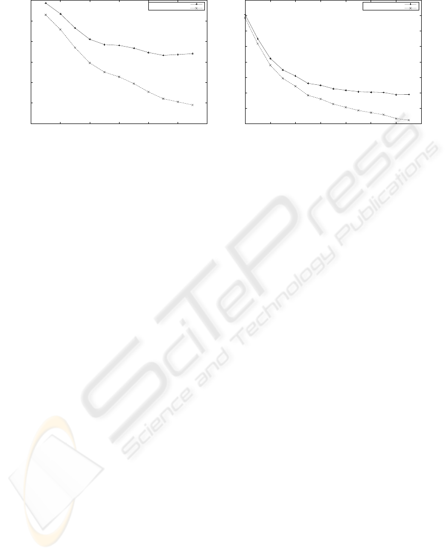
groups is listed in Table 1. Figure 4 show the two

plots of the mixture BIC scores and −2log-likelihood

values against the number of clusters for the last two

ICEIS 2004 - ARTIFICIAL INTELLIGENCE AND DECISION SUPPORT SYSTEMS

170000

175000

180000

185000

190000

195000

200000

2 4 6 8 10 12 14

BIC score & -2log-likelihood

number of clusters

BIC score & log-likelihood versus the number of clusters for 5,000 composite objects

BIC score

-2log-likelihood

330000

340000

350000

360000

370000

380000

390000

400000

410000

2 4 6 8 10 12 14 16

BIC score & -2log-likelihood

number of clusters

BIC score & log-likelihood versus the number of clusters for 9,530 composite objects

BIC score

-2log-likelihood

Figure 4: The BIC and log-likelihood versus the number of clusters for the datasets of 5,000 and 9,530 composite objects. The

ﬁrst local minimum shows the optimal numbers of clusters found by the EM algorithm are 11 and 14 clusters respectively.

groups respectively. An observation from the exper-

iments is that the optimal number of clusters found

by the algorithm is increasing as the total number of

objects increases. This can be veriﬁed from Equation

(5), where the likelihood term (O(N)) dominates the

penalty term (O(log N)) as N gets larger.

The clustering results are signiﬁcant and convinc-

ing. The count aggregates and frequency aggregates

play important roles in the clustering. The dataset

tends to be partitioned into groups that have dis-

tinct number of part objects, e.g., dwellings with

distinct number of occupants and rooms, together

with properties of distinct aggregate frequencies, e.g.,

dwellings of protestant families and dwellings in

which fewer room defects are reported. In addition,

by analysing the BIC curves in Figure 4, it is reason-

able for us to partition the whole dataset into 7 distinct

clusters at last.

6 CONCLUSION

Compared with other work, our method is a proposi-

tional approach in relational data mining. We bor-

rowed some ideas from (Fraley and Raftery, 1998;

Meil

a and Heckerman, 1998), and provide some ex-

tensions in dealing with aggregate attributes. We de-

ﬁne frequency aggregates so that both the values and

the distribution of values can be recorded for compos-

ite objects. Frequency aggregates are well applied in

computing log-likelihood distance. We also present

a method of determining the lower and upper bounds

for the EM and get good results from the experiments.

Some future work are planned to do: handling con-

tinuous attributes as well as discrete attributes; deal-

ing with missing data or data with noise; and apply-

ing relational distance measurements, e.g. (Emde and

Wettschereck, 1996) to develop a relational model-

based clustering method.

REFERENCES

Connolly, T. M. and Begg, C. E. (2002). Database Systems:

A Practical Approach to Design, Implementation, and

Management. Harlow: Addison-Wesley, third edition.

International computer science series.

zeroski, S. and Lavra

c, N. (2001). Relational Data Min-

ing. Springe-Verlag, Berlin.

zeroski, S. and Raedt, L. D. (2003). Multi-relational data

mining: a workshop report. SIGKDD Explorations,

4(2):122–124.

Emde, W. and Wettschereck, D. (1996). Relational

instance-based learning. In Proc. ICML-96, pages

122–130, San Mateo, CA. Morgan Kaufmann.

Eriksson, H.-E. and Penker, M. (1998). UML Toolkit. John

Wiley and Sons, New York.

Everitt, B. (1981). Cluster Analysis. Halsted Press: John

Wiley and Sons, New York, second edition.

Fraley, C. and Raftery, A. (1998). How many clusters?

which clustering method? answers via model-based

cluster analysis. The Computer Journal, 41(8):578–

588.

Friedman, N., Getoor, L., Koller, D., and Pfeffer, A.

(1999). Learning probabilistic relational models. In

Proc. IJCAI-99, pages 1300–1307, Stockholm, Swe-

den. Morgan Kaufmann.

Jain, A. K. and Dubes, R. C. (1988). Algorithms for Clus-

tering Data. Prentice-Hall.

Meil

a, M. and Heckerman, D. (1998). An experimen-

tal comparison of several clustering and initialization

methods. In Proc. UAI 98, pages 386–395, San Fran-

cisco, CA. Morgan Kaufmann.

Taskar, B., Segal, E., and Koller, D. (2001). Probabilis-

tic classiﬁcation and clustering in relational data. In

Nebel, B., editor, Proc. IJCAI-01, pages 870–878,

Seattle, US.

HIERARCHICAL MODEL-BASED CLUSTERING FOR RELATIONAL DATA