
AN EXPERIENCE WITH THE NEURAL NETWORK FOR
AUTO-LANDING SYSTEM OF AN AIRCRAFT
Dr. Sreenatha G. Anavatti
School of Aerospace, Civil and Mechanical Engineering, University of New South Wales at ADFA, Canberra, Australia
Dr. Choi J. Young
School of Electrical Engineering and Computer Science, Seoul National University, Seoul, Korea
Mr. Francois Pischery
Laboratoire d’Automatique, Industrielle Institut National des Sciences Appliquees, de Lyon, Villeurbanne, France
Keywords: Auto-landing, Robust Control, Neural Network, Aircraft Dynamics
Abstract: Generalization by the Neural Networks is an added advantage that can provide very good robustness and
disturbance rejection properties. By providing a sufficient number of training samples (inputs and their
corresponding outputs), a network can deal with some inputs it has never seen before. This ability makes
them very interesting for control applications because not only they can learn complicated control functions
but they are able to respond to changing or unexpected environments. Aircraft landing system provides one
such scenario wherein the flight conditions change quite dramatically over the path of descent. The present
work discusses the training of a neural network to imitate a robust controller for auto-landing of an
aircraft. The comparisons with the robust controller indicate the additional advantages of the neural
network
1 INTRODUCTION
Auto-landing is a requirement in the modern aircraft
due to the necessity for operations under all weather
conditions, whether it is civilian aircraft or military
aircraft. Considerable efforts have gone in designing
suitable control systems for enhancing the auto-
landing capability[1,5]. The auto-landing consists of
the two phases, the descent phase and the flare.
During the descent phase, the glide slope control
system guides the aircraft down a pre-determined
glide-slope. When the aircraft reaches a pre-selected
altitude, the flare control system reduces the rate of
descent and causes the aircraft to flare out and touch
down with an acceptably low rate of descent. The
control system achieves this by the control of the
flight path angle γ. It is shown in reference (John H.
Blakelock, 1991) that the automatic control of the
flight path angle without simultaneous control of the
airspeed (either manual or automatic) is practically
not possible. The combination of these three
systems provides the full longitudinal control of the
aircraft.
The dynamics of the aircraft is governed by
stability derivatives which are functions of flight
regime (speed, altitude, density, temperature, etc.).
Due to the variations in the flight regime during
landing, the dynamics of the aircraft change
considerably over the entire flight regime. Hence, a
time varying mathematical model is required. Due
to the difficulty in handling time-varying differential
equations, mathematical models at a number of
points in the descent are considered simultaneously.
This adds a large amount of uncertainty in modelling
employed in the design of flight control systems. In
addition, disturbances in terms of gusts and sensor
and actuator noise can alter the performance of
control system considerably. Hence, there is a
necessity for having robust control systems that can
handle parameter variations along with good
disturbance rejection properties. H-infinity(Ching-
Fang Lin, 1995) controller provides one such
393
G. Anavatti S., J. Young C. and Pischery F. (2004).
AN EXPERIENCE WITH THE NEURAL NETWORK FOR AUTO-LANDING SYSTEM OF AN AIRCRAFT.
In Proceedings of the Sixth International Conference on Enterprise Information Systems, pages 393-400
DOI: 10.5220/0002627603930400
Copyright
c
SciTePress

alternative. However, the complexity of the
controller can deter the implementation in practical
uses.
The present paper looks at the alternate way of
implementing the H-infinity controller by training a
neural network[2,3] to imitate this. In addition to
the imitation, the neural network is shown to have
additional properties like generalization with inputs
and better robustness properties.
Section 2 discusses the auto-landing and the
equations governing the dynamics of the aircraft.
Section 3 discusses the design of neural network to
imitate the H-infinity controller. The details of the
design of H-infinity controller are avoided to reduce
the mathematical complexity of the paper. Section 4
presents the comparison between the H-infinity and
the neural network controllers under various
conditions. The paper is concluded in section 5.
2 AIRCRAFT DYNAMICS AND
AUTO-LANDING SYSTEM
The linearized equations describing the longitudinal
motion of the aircraft are:
q
MqMMuMqM
ZgZuZZ
XgXuXu
eequ
eeu
rpmrpmu
=
+++=+−
+Θ−+=
+Θ−+=
θ
δαα
δθαα
δ
θ
α
δαα
δαα
δα
&
&
&
&
&
&
0
0
cos
cos
where, u is the change in airspeed (ft/sec), α is the
angle of attack (deg), θ is the pitch angle (deg), δ
e
is
the elevator angle (deg), δ
rpm
is the change in the
rpm of the engine (rpm), and Θ
0
is the initial Euler
angle relative to the horizontal plane. X
u,
X , Z
u
, Z ,
Z
, M
u
. M , M
,
M
q
,, M
e
, Z
e
are known as the
stability derivatives. These are functions of the
flight regime like the speed, density, altitude, etc.
These equations can be set in the State-Space form
given by,
DU
CX
Y
BUAXX
+=
+=
&
where X is the state vector, U is the input vector and
Y is the output vector.
2.1 Basic Autopilot Model
The basic autopilot is actually the pitch angle control
system. The error on θ goes through a transfer
function that stands for electronics and hydraulics.
The result is δ
e
, the elevator deflection. Then the
aircraft equations compute the associated reaction.
The outputs of the aircraft block are the change in
airspeed (u) and the pitch rate (q).
The basic autopilot includes a velocity control
system (VCS). It uses the throttle to correct the
change in airspeed (Fig. 2). The input is the change
in airspeed (u) and the output is the engine rpm
correction.
In the following,
γ
(deg) is the flight path angle.
It is actually the parameter that is being controlled
but it is never measured directly. It is linked to
θ
and
α
by:
α
θ
γ
−=
The following simulation results were obtained
with a 1 deg step command input on
θ
. The velocity
control system ensures that the direction of the flight
path angle is in the same direction as the pitching
angle (otherwise, when the aircraft is commanded to
descend, it would actually have a shallow glide up).
2.2 Glide slope control system
The glide slope controller surrounds the basic
autopilot. It computes the right input θ
comm
for the
basic autopilot so the aircraft stays on the predefined
flight path. The task of the glide slope control
system is to keep Γ = 0 so that the aircraft descends
along the desired path.
2.3 Flare Control System
As the glide slope controller, the flare controller
surrounds the aircraft/autopilot model and computes
the input
θ
comm
so the aircraft sticks with the
predetermined flight path.
Flight test data has shown that when a pilot
performs the flare from the approach glide to the
final touchdown he generally decreases his rate of
descent in an exponential manner, thus tending to
make the aircraft fly an exponential path.
For the automatic flare control, then, the aircraft
is commanded to fly an exponential path from the
initiation of the flare until touchdown. The height
above runway (h) is given by :
τ
/
0
t
ehh
−
=
h is the height (ft).
h
0
is the height at the start of the flare (ft).
τ
is the time constant (sec).
τ
and h
0
are calculated by making assumptions on
the distance between the touchdown point and the
transmitter and on the time the aircraft will take to
reach to touchdown.
ICEIS 2004 - ARTIFICIAL INTELLIGENCE AND DECISION SUPPORT SYSTEMS
394
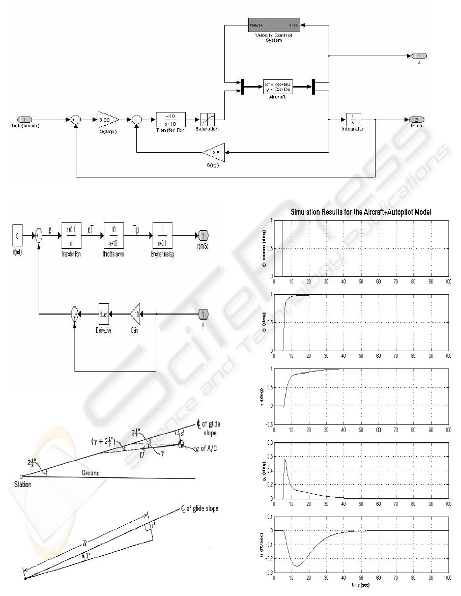
Figure 1: Basic autopilot block diagram
Figure 2: Velocity control system.
Figure 4: Geometry of Glide Slope Problem
Figure 3: Simulation Results of basic autopilot
AN EXPERIENCE WITH THE NEURAL NETWORK FOR AUTO-LANDING SYSTEM OF AN AIRCRAFT
395
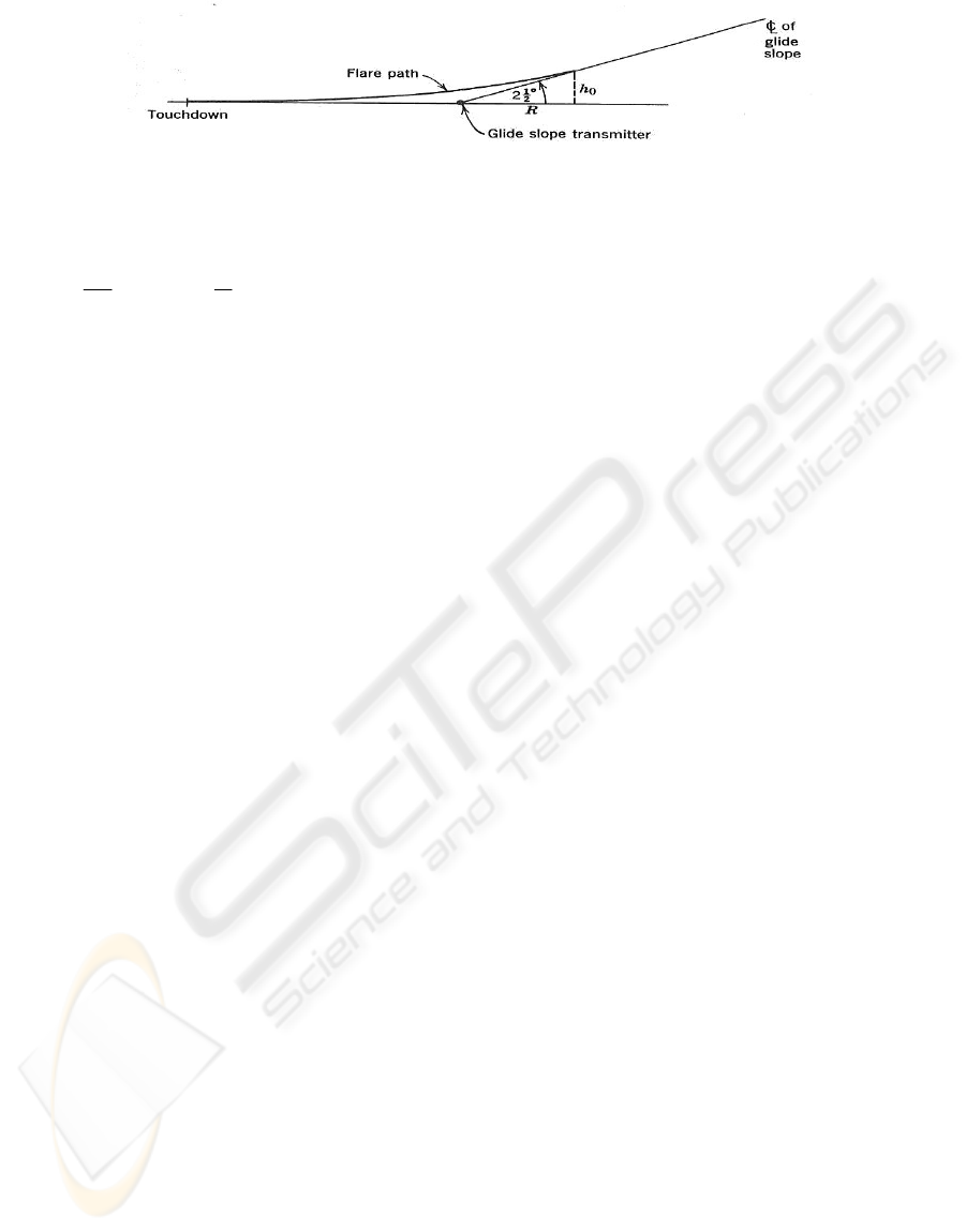
Figure 5: Geometry of the Glide Slope
As the path equation is known, the value of
h
&
(rate of descent) is known at any time :
τ
τ
τ
h
e
h
h
t
−=−=
− /
0
&
This is the command signal for the outer loop.
The coupler shown above is a conventional one that
does not have the properties of robustness. One can
design a better controller that has better robustness
properties. One such controller is the H-infinity
controller.
The H
∞
control design approach consists in
modeling uncertainties as a separate transfer
function that is combined with the plant model in a
multiplicative or additive way. This way the H
∞
controller is able to stabilize not only the nominal
model but a whole family of systems which exist in
the uncertainty region around the nominal model.
However, the complexity of the controller deters the
implementation in the practical systems.
3 NEURAL NETWORK
A feedforward network is employed in the present
work. The training of the network was performed
using the back propagation algorithm.
MATLAB(Howard Demuth et al., 2000) was
employed for doing the same. For the sake of
completeness, the training algorithm is summarized
below;
The backpropagation algorithm used in this
study was the Levenberg-Marquardt algorithm
(trainlm in MATLAB). It is one of the many
variations of the backpropagation algorithm. It was
chosen for its speed of convergence in function
approximation problems. It is inspired by the
Newton method for which the basic step is:
kkkk
gHxx
1
1
−
+
−=
where H is the Hessian matrix of the performance
index at the current values of the weights and biases
and g is the current gradient of the performance
function.
It is often complex and expensive to compute the
Hessian matrix. The Levenberg-Marquardt
algorithm avoids this calculation by approximating
the Hessian matrix as:
JJH
T
=
and by computing the gradient as:
eJg
T
=
where J is the Jacobian matrix that contains first
derivatives of the network errors with respect to the
weights and biases, and e is a vector of network
errors. The Jacobian matrix can be computed
through a standard backpropagation technique
(much less complex than computing the Hessian
matrix).
The Levenberg_Marquardt algorithm then uses
this approximation in the following Newton-like
update;
[]
eJIJJxx
TT
kk
1
1
−
+
+−=
µ
When the scalar
µ is zero, this is just Newton’s
method, using the approximate Hessian Matrix.
When
µ is large, this becomes gradient descent with
a small step size. Newton’s method is faster and
more accurate near an error minimum, so the aim is
to shift towards Newton’s method as quickly as
possible. Thus,
µ is decreased after each successful
step and increased only when a tentative step would
increase the performance function.
ICEIS 2004 - ARTIFICIAL INTELLIGENCE AND DECISION SUPPORT SYSTEMS
396
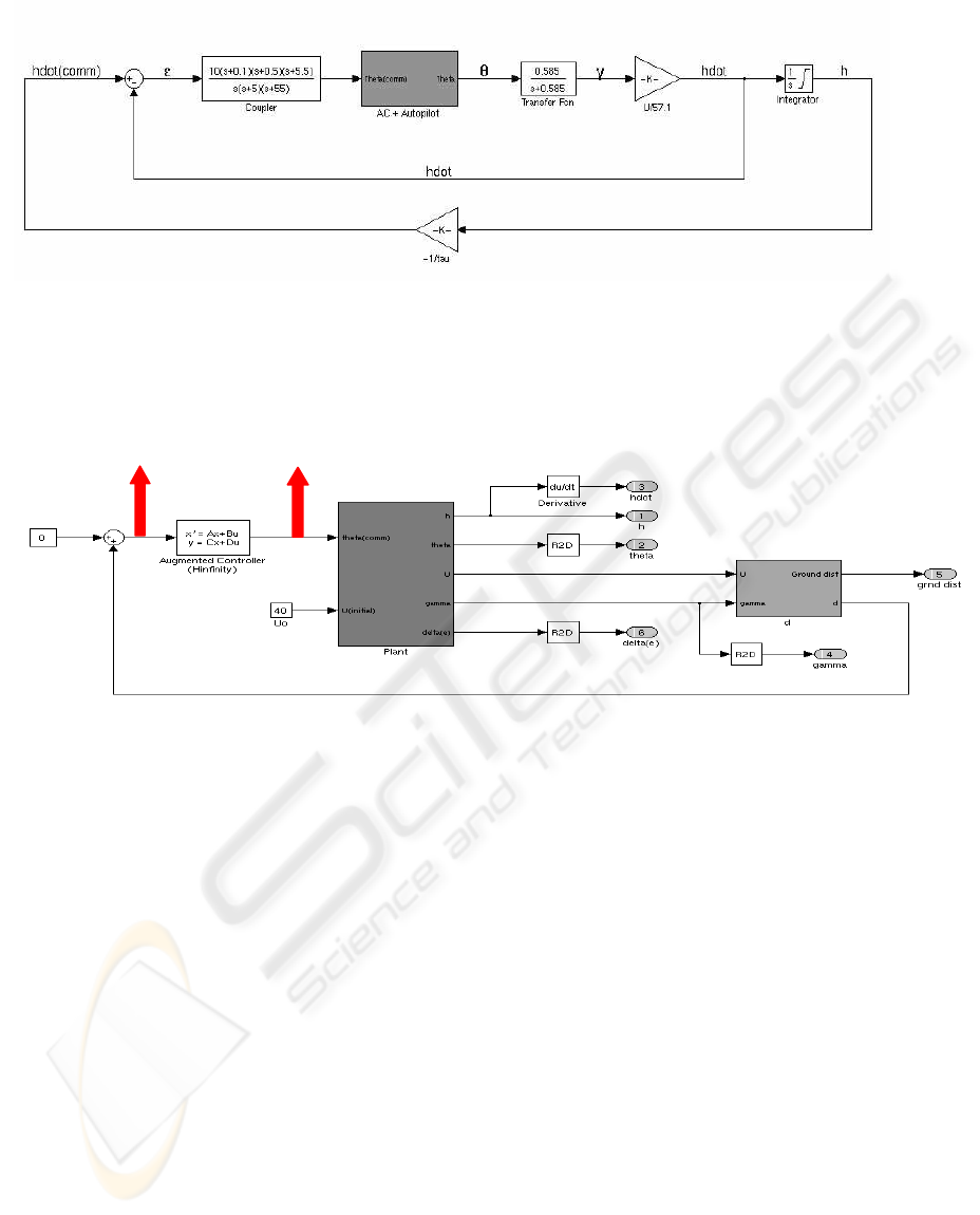
Figure 6: Flare control system
3.1 First attempt in training
Since, the network is supposed to imitate the H-
infinity controller, the training data employed was
the input and out of the H-infinity controller,as
shown in the block diagram (Figure 7).
Figure 7: Block diagram for the first configuration
At this stage, the neural network is a 3-layer
feedforward network, with the hidden layer
consisting of 5 and 3 neurons. The training set
consists of the input vector d, the distance between
the aircraft center of gravity and the ideal glide slope
and output vector, the H
∞
controller output.
The performance function did not achieve the
targeted minimum with any number of epochs.
Increasing the number of layers and neurons also did
not help the cause. Due to the ambiguity in the
relation between the input and the output, this was
happening.
3.2 Second attempt in training:
In order to remove the ambiguity, the network will
now receive two inputs: u (the airspeed change) and
γ (the flight path angle). θ
comm
(H
∞
controller output)
is still the target. In this configuration, the network is
meant to replace both the “d” block and the H
∞
controller.
This time, convergence was achieved and the
desired performance level was achieved during the
training. The numerical simulations with this
network showed that the response matches very well
with that obtained by the H-infinity controller. Since
the network was trained for a particular initial
condition (distance between the aircraft centre of
gravity and the ideal glide slope line)(in this case d
0
= 70m), when this initial condition was modified,
the network did not perform according to the
expectations. The graphs below show the evolution
of d during the landing phase: the shape stays
exactly the same and the error is brought back to
zero in the first case; in the second case the aircraft
flies along its glide slope but 30m away from it
(Figure 8). In order to correct this, the network has
to be trained with not only one set of data but several
data sets each corresponding to a different initial
condition.
As the final step in training, an extra input
neuron for the initial condition with 9 and 7 neurons
in the hidden layer were employed.
Inputs
Targets
AN EXPERIENCE WITH THE NEURAL NETWORK FOR AUTO-LANDING SYSTEM OF AN AIRCRAFT
397
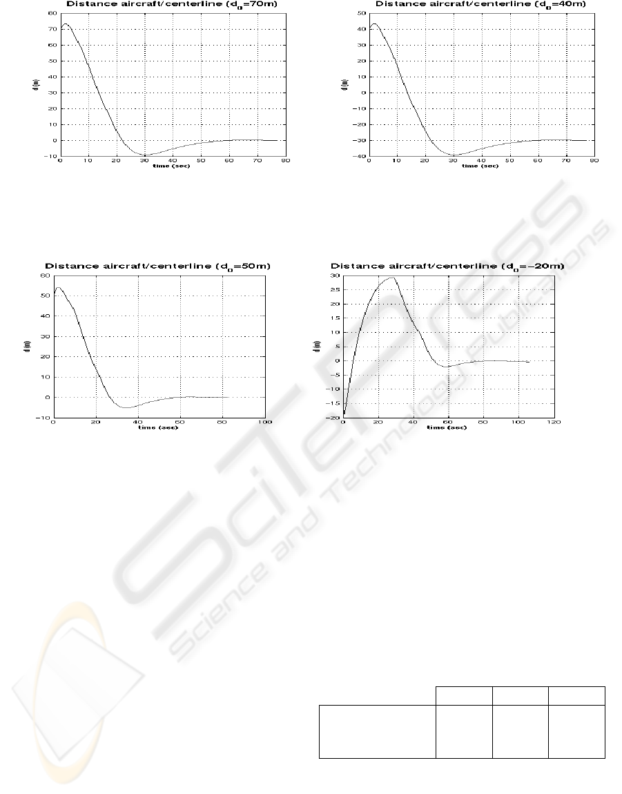
Figure 8: Neural Network behaviour for two different initial conditions
This network was trained with three data sets
corresponding to three different initial conditions: d
0
equals to 100, 50 and -20m. After 500 epochs, the
mean square error is equal to 2.4e-6. The simulation
shows that the neural networks behavior is
satisfactory for the initial conditions included in the
training.
Figure 9: Neural Network results for two different initial conditions (final network).
However, when other initial conditions were tried
out, the performance was not good. Once again this
is attributed to the ambiguity and hence, an
additional input (the integrated value of distance, d)
was employed. With this, the final training was
carried out with data for initial conditions of d
0
= -
100, -90, -80, …, 90, 100m. The final network was a
four layer network with 10 neurons per hidden layer.
In addition, another network with 11 neurons per
hidden layer was also trained. The results of
comparison of these two networks with H-infinity
controller indicate the generalization property of the
network as well as the effect of architecture on the
robustness.
4 PERFORMANCE AND
ROBUSTNESS
The performance of the controller for auto-landing is
measured through the global accuracy of the landing
system. Robustness evaluation is based on three
tests: sensitivity to modeling errors, disturbance
rejection and sensitivity to sensor noise. The
following paragraphs compare the results for the
three controllers. For convenience, the H-infinity
controller and the neural networks will respectively
be called H
∞
, NN
10
and NN
11
here afterwards.
4.1 Accuracy
The neural networks were trained for initial
conditions varying within [-100;+100]. For several
initial conditions from this range and for each
controller, d
touchdown
is measured (Figure 10). For
each controller, the maximum gap, the average gap
and the standard deviation of the values were
computed. The results are given by;
Hinf NN10 NN11
Maximum (m)
0.272 0.346
0.209
Average (m)
-0.042
0.038
-0.148
Stand. Dev.
0.101 0.146
0.078
These values show that even though NN
11
has
the highest average gap, it is the most interesting
controller here. It is very constant (low standard
deviation) and its maximum error is smaller.
ICEIS 2004 - ARTIFICIAL INTELLIGENCE AND DECISION SUPPORT SYSTEMS
398
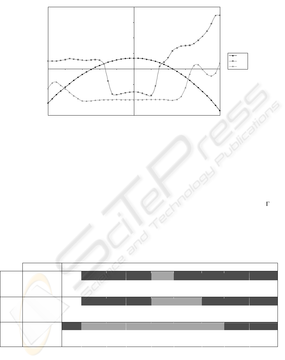
Figure 10 Controller Accuracy as a function of simulation initial conditions.
4.2 Sensitivity to uncertainty and
modeling errors
Modeling errors arise due to the simplifying
assumptions in mathematical modelling. Along with
this, due to the variations in the flight conditions, the
stability derivatives governing the dynamics of the
aircraft change. Hence, there is a necessity to
validate the controller against these.
Numerical simulations were carried out by
varying all the parameters of the A matrix by a
certain percentage indicating the worst case scenario
The controllers were tested in the following
configurations:
the stability derivatives are 5, 8, 10 and 11%
bigger,
the stability derivatives are 10, 15, 16 and
17% smaller.
For a certain amount of change in the A matrix,
the natural frequencies governing the dynamics of
the aircraft change. The aim is to define the range
of natural frequencies in which each controller stays
effective. Like before, the effectiveness is measured
through d
touchdown
.
It is assumed that 50cm is the maximum
acceptable d
touchdown
. With a glide slope angle ( ) of
4°, that would mean a ground distance of about 7m
between ideal and actual touchdown points. So the
net would have to be 14m long which seems about
right. The green zones indicate that according to this
criteria, the controller kept the aircraft in the net.
The red zones means the aircraft would have missed
it.
Change -17% -16% -15% -10% 0% 5% 8% 10% 11%
Max (m)
0.427 0.468 0.516 0.272 0.506 0.897 1.278 1.508
Avg (m)
-0.017 -0.034
-0.088 -0.042 -0.062 -0.137 -0.223 -0.279
Hinf
Std
0.122 0.132 0.144 0.101 0.133 0.215 0.302 0.356
Max (m)
7.541 5.986 2.166 0.346 0.239 0.809 1.404 1.697
Avg (m)
-4.895 -4.021
-1.610
0.038 -0.037
-0.115 -0.202 -0.259
NN10
Std
1.659 1.344 0.299 0.146 0.090 0.140 0.266 0.343
Max (m)
24.406
0.101 0.109 0.140 0.209 0.136 0.477 1.036 1.457
Avg (m)
1.269
-0.009 -0.010
-0.028
-0.148 -0.084
-0.110 -0.166 -0.216
NN11
Std
5.557
0.031 0.031 0.038 0.078 0.023 0.084 0.203 0.299
These results show the superiority of NN
11
. Its
maximum distances at touchdown are always
smaller than the others and as shown by the green
zones, its range of effectiveness is wider. NN
11
is
valid from –16% to +8%, which gives [1.922;4.303]
as natural frequency validity range, whereas H
∞
is
not even valid from –10% to +5%, which gives the
validity range [2.059;4.184]. In addition
, NN
11
average errors are very small and actually
-0,300
-0,200
-0,100
0,000
0,100
0,200
0,300
0,400
-100 -80 -60 -40 -20 0 20 40 60 80 100
Simulation initial condition (m)
Gap @ touchdown (m)
Hinf
NN10
NN11
AN EXPERIENCE WITH THE NEURAL NETWORK FOR AUTO-LANDING SYSTEM OF AN AIRCRAFT
399
improve a little bit with parameter variation. Finally,
its standard deviation indicate that it is by far the
most consistent of the tested controllers.
The neural network was trained with samples
created by H
∞
only. So the neural network not only
does the job of what H
∞
’s does, but does it better.
The neural network is able to compensate for a
bigger change. As this result was reached with a
training set including only data for the ideal plant
configuration, it is very possible that additional
training (with data from several controllers and
several plant configurations) enhances the
robustness of NN
11
.
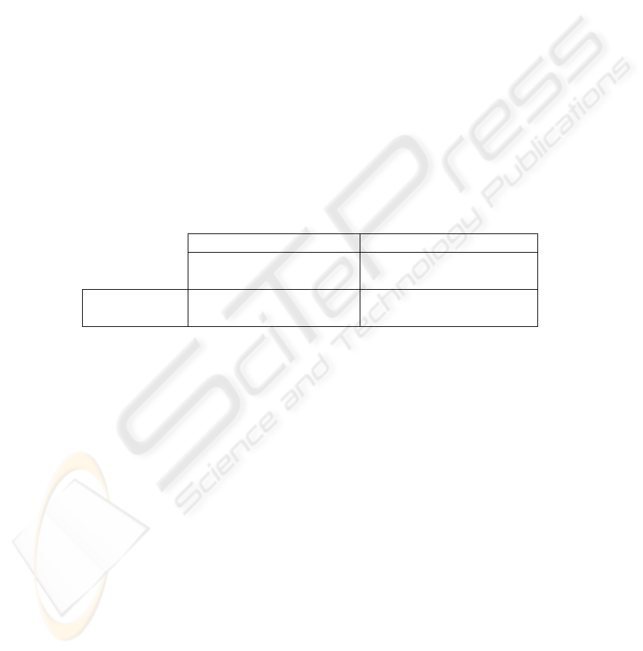
4.3 Disturbance rejection
In general, the disturbances can be on the actuator
side or the sensor side. Since the control surfaces (in
this case elevator) are the actuators for an aircraft,
the presence of atmospheric disturbances can be
translated as equivalent disturbances on these
aerodynamic control surfaces. The aircraft should
be able to withstand these disturbances. To model
external disturbances, random signals of various
amplitude were added to δ
e
, the elevator deflection
and simulations were conducted. Three cases of
10%, 25% and 50% of δ
e
curent amplitude are
considered. In each of these cases and for each
controller, the entire flight path was compared to the
clean flight path (without disturbances). For each
time step, the difference between the clean and noisy
flight paths was computed. Based on these
difference numbers, an average difference and the
standard deviation were computed. Because this
time the entire flight path is monitored and not just
the gap at touchdown, this test was not run for
several initial conditions but just for d
0
= 50m. The
table below summarises the results.
H
∞
appears to have a slightly better resistance to
disturbances when their amplitude grows. But
globally, NN
11
does not have a bad behavior. Its
numbers are very much comparable to those of H
∞
.
We believe that by including noise or noisy inputs in
the training set, the neural network should improve
its filtering capabilities significantly. Unfortunately,
the lack of time prevented us from going any further
in this direction.
Hinf NN11
Difference (m) Difference (m)
10%
25%
50%
10%
25%
50%
Average (m)
0,005 0,012
0,032
-0,002 0,016
0,120
Stand. Dev.
0,124
0,294
0,832 0,098 0,329
0,836
5 CONCLUDING REMARKS
This paper discusses the experience in training a
neural network to imitate a complex robust
controller for auto-landing of aircraft, a major
requirement for the present day aircraft. The various
steps in achieving the desired training and the results
of the comparison are presented in graphical as well
as tabular form. To verify the performance of the
controller, both accuracy and robustness are
considered. The neural network seems to do a better
job than the controller used for its training due to the
generalization nature of these networks. Additional
training with noisy data can improve the filtering
characteristics of these networks in a significantly
thus combining the efforts of the filter and the
controller in a single network.
REFERENCES
John H. Blakelock, (1991), Automatic Control of Aircraft
and Missiles.
Marilyn McCord Nelson, W.T. Illingworth, (1991), A
Practical Guide to Neural Nets.
William E. Faller, Scott J. Schreck, (1996), Neural
Networks : Applications and Opportunities in
Aeronautics, Progress in Aerospace Sciences, Vol. 32,
Issue 5.
Howard Demuth, Mark Beale, (2000), Neural Network
Toolbox User’s Guide, Version 4 (Release 12).
Louis V. Schmidt, (1998), Introduction to Aircraft Flight
Dynamics, AIAA Education Series.
Ching-Fang Lin, (1995), Advanced Control Systems
Design, PTR Prentice Hall
.
ICEIS 2004 - ARTIFICIAL INTELLIGENCE AND DECISION SUPPORT SYSTEMS
400
