NEW ENERGETIC SELECTION PRINCIPLE

IN DIFFERENTIAL EVOLUTION

Vitaliy Feoktistov

Centre de Recherche LGI2P, Site EERIE, EMA

Parc Scientiﬁque Georges Besse, 30035 Nimes, France

Stefan Janaqi

Centre de Recherche LGI2P, Site EERIE, EMA

Parc Scientiﬁque Georges Besse, 30035 Nimes, France

Keywords:

differential evolution, evolutionary algorithms, heuristics, optimization, selection.

Abstract:

The Differential Evolution algorithm goes back to the class of Evolutionary Algorithms and inherits its phi-

losophy and concept. Possessing only three control parameters (size of population, differentiation and recom-

bination constants) Differential Evolution has promising characteristics of robustness and convergence. In

this paper we introduce a new principle of Energetic Selection. It consists in both decreasing the population

size and the computation efforts according to an energetic barrier function which depends on the number of

generation. The value of this function acts as an energetic ﬁlter, through which can pass only individuals with

lower ﬁtness. Furthermore, this approach allows us to initialize the population of a sufﬁcient (large) size. This

method leads us to an improvement of algorithm convergence.

1 INTRODUCTION

Evolutionary Algorithms increasingly become the

primary method of choice for optimization problems

that are too complex to be solved by deterministic

techniques. They are universal, robust, easy to use

and inherently parallel. The huge number of appli-

cations and continuous interest prove it during sev-

eral decades (Heitk

otter and Beasley, 2000; Beasley,

1997). In comparison with the deterministic methods

Evolutionary Algorithm require superﬁcial knowl-

edge about the problem being solved. Generally, the

algorithm only needs to evaluate the cost function for

a given set of input parameters. Nevertheless, in most

cases such heuristics take less time to ﬁnd the opti-

mum than, for example, gradient methods. One of the

latest breakthroughs in the evolutionary computation

is the Differential Evolution algorithm.

2 DIFFERENTIAL EVOLUTION

Differential Evolution (DE) is a recently invented

global optimization technique (Storn and Price,

1995). It can be classiﬁed as an iterative stochas-

tic method. Enlarging the Evolutionary Algorithms’

group, DE turns out to be one of the best population-

based optimizers (Storn and Price, 1996; Feoktis-

tov and Janaqi, 2004c; Feoktistov and Janaqi, 2004a;

Feoktistov and Janaqi, 2004b). In the following lines

we give a brief description of DE algorithm.

An optimization problem is represented by a set of

variables. Let these variables form a D-dimensional

vector in continuous space X = (x

, . . . , x

) ∈

. Let there be some criterion of optimization

f : IR

→ IR, usually named ﬁtness or cost function.

Then the goal of optimization is to ﬁnd the values of

the variables that minimize the criterion, i.e. to ﬁnd

∗

: f(X

∗

) = min

f(X) (1)

Often, the variables satisfy boundary constraints

L ≤ X ≤ H : L, H ∈ IR

(2)

As all Evolutionary Algorithms, DE deals with a

population of solutions. The population IP of a gener-

ation g has NP vectors, so-called individuals of pop-

ulation. Each such individual represents a potential

optimal solution.

= X

, i = 1, . . . , N P (3)

In turn, the individual contains D variables, so called

genes.

= x

i,j

, j = 1, . . . , D (4)

The population is initialized by randomly generat-

ing individuals within the boundary constraints,

= x

i,j

= rand

i,j

· (h

− l

) + l

(5)

Feoktistov V. and Janaqi S. (2004).

NEW ENERGETIC SELECTION PRINCIPLE IN DIFFERENTIAL EVOLUTION.

In Proceedings of the Sixth International Conference on Enterprise Information Systems, pages 29-35

DOI: 10.5220/0002631200290035

 SciTePress

where rand function generates values uniformly in

the interval [0, 1].

Then, for each generation the individuals of the

population are updated by means of a reproduction

scheme. Thereto for each individual ind a set of other

individuals π is randomly extracted from the popula-

tion. To produce a new one the operations of Differ-

entiation and Recombination are applied one after an-

other. Next, the Selection is used to choose the best.

Now brieﬂy consider these operations.

Here, we show the typical model of the Differenti-

ation, others can be found in (Feoktistov and Janaqi,

2004a; Feoktistov and Janaqi, 2004c). For that, three

different individuals π = {ξ

, ξ

} are randomly

extracted from a population. So, the result, a trial in-

dividual, is

τ = ξ

+ F · (ξ

− ξ

) , (6)

where F > 0 is the constant of differentiation.

After, the trial individual τ is recombined with up-

dated one ind. The Recombination represents a typ-

ical case of a genes’ exchange. The trial one inherits

genes with some probability. Thus,

if rand

< Cr

ind

otherwise

(7)

where j = 1, . . . , D and Cr ∈ [0, 1) is the constant

of recombination.

The Selection is realized by comparing the cost

function values of updated and trial individuals. If

the trial individual better minimizes the cost function,

then it replaces the updated one.

ind =

ω if f(ω) ≤ f(ind)

ind otherwise

(8)

Notice that there are only three control parameters

in this algorithm. These are N P – population size, F

and Cr – constants of differentiation and recombina-

tion accordingly. As for the terminal conditions, one

can either ﬁx the number of generations g

max

or a de-

sirable precision of a solution V T R (value to reach).

The pattern of DE algorithm is presented in Algo-

rithm 1.

3 DIFFERENTIATION

Differentiation occupies a quite important position in

the reproduction cycle. So, we try to analyze it in

detail.

Geometrically, Differentiation consists in two si-

multaneous operations: the ﬁrst one is the choice of

a Differentiation’s direction and the second one is the

calculation of a step length in which this Differenti-

ation performs. From the optimization point of view

we have to answer the next two questions:

Algorithm 1 Differential Evolution

Require: F, Cr, N P – control parameters

initialize IP

← {ind

, . . . , ind

}

evaluate f(IP

)

while (terminal condition) do

for all ind ∈ IP

→ π = {ξ

, ξ

, . . . , ξ

}

τ ← Diff erentiate(π, F )

ω ← Recombine(τ, Cr)

ind ← Select(ω, ind)

end for

g ← g + 1

end while

1. How to choose the optimal direction from all avail-

able ones?

2. What step length is necessary in order to better

minimize the cost function along the chosen direc-

tion?

Let us remind that the principle of Differentiation

is based on a random extraction of several individuals

from the population and the geometrical manipulation

of them.

Possible directions of Differentiation entirely de-

pend on the disposition of extracted individuals. Also,

their disposition inﬂuences the step length. Further-

more by increasing either the size of population or

the number of extracted individuals we augment the

diversity of possible directions and the variety of step

lengths. Thereby we intensify the exploration of the

search space. But on the other hand, the probability

to ﬁnd the best combination of extracted individuals

goes considerably down.

Example. We take the typical differentiation strat-

egy u = x

+ F · (x

− x

), where for each cur-

rent individual three other individuals are randomly

extracted from the population.

• In the ﬁrst case we suppose that the population

consists only of four individuals. So there are

(4 − 1)(4 − 2)(4 − 3) = 3 · 2 · 1 = 6 possible di-

rections and 6 possible step lengths. Imagine then

that only one combination gives the best value of

the cost function. Therefore the probability to ﬁnd

it, is 1/6.

• In the second case the population size is equal to

ﬁve individuals. It gives (5 − 1)(5 − 2)(5 − 3) =

4 · 3 · 2 = 24 directions and as many step lengths.

But, in this case, the probability to ﬁnd the best

combination is much less – 1/24.

If we choose another strategy consisting of two ran-

domly extracted individuals, u = x

+ F · (x

− x

)

for example, then for the population size of ﬁve in-

dividuals the diversity of possible directions and step

ICEIS 2004 - ARTIFICIAL INTELLIGENCE AND DECISION SUPPORT SYSTEMS

lengths is equal now to (5−1)(5−2) = 12 (two times

less then in the previous case).

As we can see only two factors control the capa-

bility of the search space exploration. These are the

population size N P and the number of randomly ex-

tracted individuals k in the strategy. In the case of

the consecutive extraction of individuals the depen-

dence of the potential individuals diversity from both

the population size and the number of extracted indi-

viduals is shown in the Formula 9.

f(NP, k) =

i=1

(NP − i) (9)

But, where is the compromise between the covering

of the search space (i.e. the diversity of directions and

step lengths) and the probability of the best choice?

This question makes us face with a dilemma that was

named ”The Dilemma of the search space exploration

and the probability of the optimal choice”.

During the evolutionary process the individuals

learn the cost function surface (Price, 2003). The step

length and the difference direction adapt themselves

accordingly. In practice, the more complex the cost

function is, the more exploration is needed. The bal-

anced choice of N P and k deﬁnes the efﬁciency of

the algorithm.

4 ENERGETIC APPROACH

We introduce a new energetic approach which can be

applied to population-based optimization algorithms

including DE. This approach may be associated with

the processes taking place in physics.

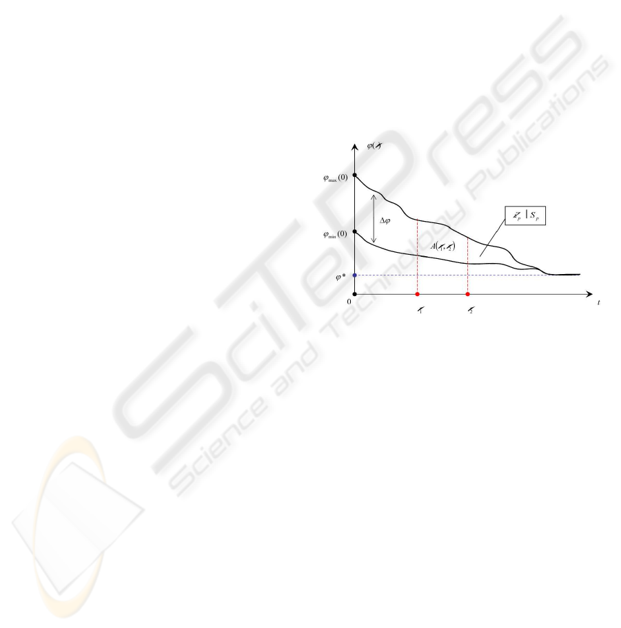
Let there be a population IP consisting of NP in-

dividuals. Let us deﬁne the potential of individual

as its cost function value ϕ = f(ind). Such poten-

tial shows the remoteness from the optimal solution

∗

= f (ind

∗

), i.e. some energetic distance (poten-

tial) that should be overcome to reach the optimum.

Then, the population can be characterized by supe-

rior and inferior potentials ϕ

max

= max f (ind

) and

min

= min f (ind

). As the population evolves the

individuals take more optimal energetic positions, the

closest possible to the optimum level. So if t → ∞

then ϕ

max

(t) → ϕ

min

(t) → ϕ

∗

, where t is an el-

ementary step of evolution. Approaching the opti-

mum, apart from stagnation cases, can be as well ex-

pressed by ϕ

max

→ ϕ

min

or (ϕ

max

− ϕ

min

) → 0.

By introducing the potential difference of population

4ϕ(t) = ϕ

max

(t) − ϕ

min

(t) the theoretical condi-

tion of optimality is represented as

4ϕ(t) → 0 (10)

In other words, the optimum is achieved when the po-

tential difference is closed to 0 or to some desired

precision ε. The value 4ϕ(t) is proportional to the

algorithmic efforts, which are necessary to ﬁnd the

optimal solution.

Thus, the action A done by the algorithm in order

to pass from one state t

to another t

A(t

, t

) =

4ϕ(t)dt (11)

We introduce then the potential energy of popula-

tion E

that describes total computational expenses.

∞

4ϕ(t)dt (12)

Notice that the equation (12) graphically repre-

sents the area S

between two functions ϕ

max

(t) and

min

(t).

Figure 1: Energetic approach.

Let us remind that our purpose is to increase the

speed of algorithm convergence. Logically, the con-

vergence is proportional to computational efforts. It is

obvious the less is potential energy E

the less com-

putational efforts are needed. Thus, by decreasing the

potential energy E

≡ S

we augment the conver-

gence rate of the algorithm. Hence, the convergence

increasing is transformed into a problem of potential

energy minimization (or S

minimization).

∗

= min

4ϕ(t)

(4ϕ(t)) (13)

5 NEW ENERGETIC SELECTION

PRINCIPLE

5.1 The Idea

We apply the above introduced Energetic Approach to

the DE algorithm. As an elementary evolution step t

we choose a generation g.

NEW ENERGETIC SELECTION PRINCIPLE IN DIFFERENTIAL EVOLUTION

In order to increase the convergence rate we min-

imize the potential energy of population E

(Fig.1).

For that a supplementary procedure is introduced at

the end of each generation g. The main idea is to

replace the superior potential ϕ

max

(g) by so called

energetic barrier function β(g). Such function artiﬁ-

cially underestimates the potential difference of gen-

eration 4ϕ(g).

β(g) − ϕ

min

(g) ≤ ϕ

max

(g) − ϕ

min

(g)

⇔ β(g) ≤ ϕ

max

(g), ∀g ∈ [1, g

max

]

(14)

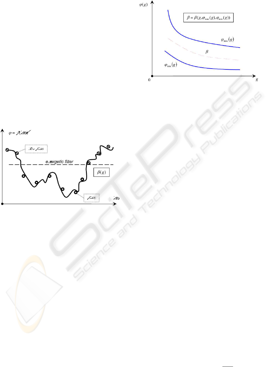
From an algorithmic point of view this function

β(g) serves as an energetic ﬁlter for the individuals

passing into the next generation. Thus, only the indi-

viduals with potentials less than the current energetic

barrier value can participate in the next evolutionary

cycle (Fig.2).

Figure 2: Energetic ﬁlter.

Practically, it leads to the decrease of the popula-

tion size NP by rejecting individuals such that:

f(ind) > β(g) (15)

5.2 Energetic Barriers

Here, we show some examples of the energetic barrier

function. At the beginning we outline the variables

which this function should depend on. Firstly, this is

the generation variable g, which provides a passage

from one evolutionary cycle to the next. Secondly, it

should be the superior potential ϕ

max

(g) that presents

the upper bound of the barrier function. And thirdly,

it should be the inferior potential ϕ

min

(g) giving the

lower bound of the barrier function (Fig.3).

Linear energetic barriers. The simplest example

is the use of a proportional function. It is easy to ob-

tain by multiplying either ϕ

min

(g) or ϕ

max

(g) with

a constant K.

Figure 3: Energetic barrier function.

In the ﬁrst case, the value ϕ

min

(g) is always stored

in the program as the current best value of the cost

function. So, the energetic barrier looks like

(g) = K · ϕ

min

(g), K > 1 (16)

The constant K is selected to satisfy the energetic bar-

rier condition (14).

In the second case, a little procedure is necessary to

ﬁnd superior potential (maximal cost function value

of the population) ϕ

max

(g). Here, the energetic bar-

rier is

(g) = K · ϕ

max

(g), K < 1 (17)

K should not be too small in order to provide a

smooth decrease of the population size NP .

An advanced example would be a superposition of

the potentials.

(g) = K · ϕ

min

(g) + (1 − K) · ϕ

max

(g) (18)

So, with 0 < K < 1 the energetic barrier function is

always found between the potential functions. Now,

by adjusting K it is easier to get the smoothed re-

duction of the population without condition violation

(14). Examples of the energetic barrier functions are

shown on the ﬁgure (Fig.4).

Nonlinear energetic barriers. As we can see the

main difﬁculty of using the linear barriers appears

when we try to deﬁne correctly the barrier function in

order to provide a desired dynamics of the population

reduction. Taking into consideration that ϕ

max

→

min

when the algorithm converges locally, the ideal

choice for the barrier function is a function which be-

gins at a certain value between ϕ

min

(0) and ϕ

max

(0)

and converges to ϕ

max

Thereto, we propose an exponential function K(g)

K(g) = K

+ (K

− K

) · e

(

−

max

·g

)

(19)

ICEIS 2004 - ARTIFICIAL INTELLIGENCE AND DECISION SUPPORT SYSTEMS

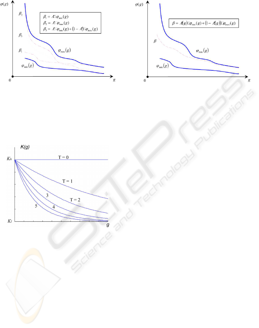
Figure 4: Linear energetic barriers.

This function, inspired by the color-temperature de-

pendence from Bernoulli’s low, smoothly converges

from K

to K

. The constant T , so called temper-

ature, controls the convergence rate. The functional

dependence on the temperature constant K(T ) is rep-

resented on the ﬁgure (Fig.5).

Figure 5: Exponential function K(g, T ).

By substituting the constant K in the equations (16-

18) for the exponential function (19) we can supply

the energetic barrier function with improved tuning

(Fig.6).

5.3 Advantages

Firstly, such principle of energetic selection permits

to initialize the population of a sufﬁciently large size.

This fact leads to better (careful) exploration of a

search space during the initial generations as well as

it increases the probability of ﬁnding the global opti-

mum.

Secondly, the introduction of the energetic barrier

function decreases the potential energy of the popula-

tion and thereby increases the algorithm rate.

Thirdly, a double selection principle is applied. The

ﬁrst one is a usual DE selection for each individual

Figure 6: Nonlinear energetic barrier.

of a population. Here, there is no reduction of the

population size. And the second one is a selection of

the best individuals which pass in the next generation,

according to the energetic barrier function. It leads to

the reduction of the population size.

Remark. Notice that a considerable reduction of

the population size occurs at the beginning of the

evolutionary process. For more efﬁcient exploitation

of this fact a population should be initialized with

greatly larger size N P

than usually. Then, when the

population shrinks to a certain size NP

, it is neces-

sary to stop the energetic selection procedure. This

forced stopping is explained by possible stagnation

and not enough efﬁcient search in a small size pop-

ulation. In fact, the ﬁrst group of generations locates

a set of promising zones. The selected individuals are

conserved in order to make a thorough local search in

these zones.

6 COMPARISON OF RESULTS

In order to test our approach we chose three test func-

tions (20) from a standard test suite for Evolutionary

Algorithms (Whitley et al., 1996). The ﬁrst two

functions, Sphere f

and Rosenbrock’s function f

are classical De Jong testbads (Jong, 1975). Sphere

is a ”dream” of every optimization algorithm. It

is smooth, unimodal and symmetric function. The

performance on the Sphere function is a measure

of the general efﬁciency of the algorithm. Whereas

the Rosenbrock’s function is a nightmare. It has a

very narrow ridge. The tip of the ridge is very sharp

and it runs around a parabola. The third function,

Rotated Ellipsoid f

, is a true quadratic non separable

optimization problem.

NEW ENERGETIC SELECTION PRINCIPLE IN DIFFERENTIAL EVOLUTION

(X) =

i=1

(X) = 100(x

− x

)

+ (1 − x

)

(X) =

i=1





j=1





(20)

We ﬁxed the differentiation F and recombination

Cr constants to be the same for all functions. F =

0.5. Recombination Cr = 0 (there is no recombina-

tion) in order to make the DE algorithm rotationally

invariant (Salomon, 1996; Price, 2003). The terminal

condition of algorithm is a desirable precision of op-

timal solution V T R (value to reach). It is ﬁxed for

all tests as V T R = 10

−6

. We count the number of

function evaluations NF E needed to reach the V T R.

The initial data are shown in the Table 6.

Table 1: Initial test data.

D NP NP

1 3 30 90 25 0.50

2 2 40 120 28 0.75

3 20 200 600 176 0.15

For DE with energetic selection principle the ini-

tial population size was chosen three times larger than

in the classical DE scheme: N P

= 3 · NP . The

forced stopping was applied if the current population

became smaller than NP . Hence NP

≤ NP . As

an energetic barrier function the linear barrier β

(g)

was selected (18). So, K is an adjusting parameter

for barrier tuning, which was found empirically. D is

the dimension of the test functions.

The average results of 10 runs for both the classical

DE scheme and DE with energetic selection principle

are summarized in the Table 2.

Table 2: Comparison the classical DE scheme (cl) and DE

with energetic selection principle (es).

NF E

δ, %

1 1088.7 912.4 16,19

2 1072.9 915.3 14,69

3 106459.8 94955.6 10,81

The numbers of function evaluations (NF E’s)

were compared. It is considered that NF E

value

is equal to 100% therefore the relative convergence

amelioration in percentage wise can be deﬁned as

δ = 1 −

NF E

(21)

Thus, δ may be interpreted as the algorithm improve-

ment.

Remark. We tested DE with a great range of other

functions. The stability of results was observed. So,

in order to demonstrate our contribution we have gen-

erated only 10 populations for each test function rely-

ing on the statistical correctness. Nevertheless farther

theoretical work and tests are necessary.

7 CONCLUSION

The variation of the population size of population-

based search procedures presents a rather promising

trend. In this article we have examined its decrease.

The proposed energetic approach explains a theoret-

ical aspect of such population reduction. The efﬁ-

ciency of the new energetic selection principle based

on this energetic approach is illustrated by the exam-

ple of the DE algorithm. The given innovation pro-

vides more careful exploration of a search space and

leads to the convergence rate improvement. Thus,

the probability of the global optimum ﬁnding is in-

creased. Further works are carried on the methods of

increasing the population size.

REFERENCES

Beasley, D. (1997). Possible applications of evolution-

ary computation. In B

ack, T., Fogel, D. B., and

Michalewicz, Z., editors, Handbook of Evolutionary

Computation, pages A1.2:1–10. IOP Publishing Ltd.

and Oxford University Press, Bristol, New York.

Feoktistov, V. and Janaqi, S. (2004a). Generalization of the

strategies in differential evolutions. In 18th Annual

IEEE International Parallel and Distributed Process-

ing Symposium. IPDPS – NIDISC 2004 workshop,

page (accepted), Santa Fe, New Mexico – USA. IEEE

Computer Society.

Feoktistov, V. and Janaqi, S. (2004b). Hybridization of

differential evolution with least-square support vec-

tor machines. In Proceedings of the Annual Machine

Learning Conference of Belgium and The Nether-

lands. BENELEARN 2004., pages 53–57, Vrije Uni-

versiteit Brussels, Belgium.

Feoktistov, V. and Janaqi, S. (2004c). New strategies in dif-

ferential evolution. In Parmee, I., editor, 6-th Interna-

tional Conference on Adaptive Computing in Design

and Manufacture, ACDM 2004, page (accepted), Bris-

tol, UK. Engineers House, Clifton, Springer-Verlag

Ltd.(London).

ICEIS 2004 - ARTIFICIAL INTELLIGENCE AND DECISION SUPPORT SYSTEMS

Heitk

otter, J. and Beasley, D. (2000). Hitch Hiker’s Guide

to Evolutionary Computation: A List of Frequently

Asked Questions (FAQ).

Jong, K. A. D. (1975). An analysis of the behavior of a class

of genetic adaptive systems. PhD thesis, University of

Michigan.

Price, K. (2003). New Ideas in Optimization, Part 2: Dif-

ferential Evolution. McGraw-Hill, London, UK.

Salomon, R. (1996). Re-evaluating genetic algorithm per-

formance under coordinate rotation of benchmark

functions: A survey of some theoretical and practical

aspects of genetic algorithms. BioSystems, 39:263–

278.

Storn, R. and Price, K. (1995). Differential evolution - a

simple and efﬁcient adaptive scheme for global opti-

mization over continuous spaces. Technical Report

TR-95-012, International Computer Science Institute,

Berkeley, CA.

Storn, R. and Price, K. (1996). Minimizing the real func-

tions of the ICEC’96 contest by differential evolu-

tion. In IEEE International Conference on Evolu-

tionary Computation, pages 842–844, Nagoya. IEEE,

New York, NY, USA.

Whitley, D., Rana, S. B., Dzubera, J., and Mathias, K. E.

(1996). Evaluating evolutionary algorithms. Artiﬁcial

Intelligence, 85(1-2):245–276.

NEW ENERGETIC SELECTION PRINCIPLE IN DIFFERENTIAL EVOLUTION