A Pitfall in Determining the

Optimal Feature Subset Size

Juha Reunanen

ABB, Web Imaging Systems

P.O. Box 94, 00381 Helsinki, Finland

Abstract. Feature selection researchers often encounter a p eaking phe-

nomenon: a feature subset can be found that is smaller but still enables

building a more accurate classiﬁer than the full set of all the candidate

features. However, the present study shows that this peak may often be

just an artifact due to the still too common mistake in pattern recogni-

tion — that of not using an independent test set.

Keywords: Peaking phenomenon, feature selection, overﬁtting, accuracy

estimation

1 Introduction

Given a classiﬁcation (or regression) problem and a potentially large set of can-

didate features, the feature selection problem is about ﬁnding useful subsets

of these features. Doing this selection automatically has been a research topic

already for decades.

Why select only a subset of the features available for training an automatic

classiﬁer? Many reasons can be found, such as the following [see e.g. 1, 2, 3]:

1. The accuracy of the classiﬁer may increase.

2. The cost of acquiring the feature values is reduced.

3. The resulting classiﬁer is simpler and faster.

4. Domain knowledge is obtained through the identiﬁcation of the salient fea-

tures.

Of these reasons, this pap er discusses the ﬁrst one. Finding a feature subset

that increases the accuracy of the classiﬁer to be built can indeed be seen as an

important motivation for many feature selection studies [2, 4, 5, 6, 7].

The assumption that removing the bad features increases the accuracy derives

from the well-known diﬃculty of coping with an increasing number of features,

which is often referred to as the curse of dimensionality [8, p. 94]. This diﬃculty

suggests the peaking phenomenon: the peak of the classiﬁcation accuracy lies

somewhere between using no features and using all the available features.

If the full probability distributions of the features with respect to the diﬀerent

classes were known, then one could in theory derive an optimal classiﬁcation

b ehavior called the Bayes rule, which would exhibit no peaking at all [see e.g.

Reunanen J. (2004).

A Pitfall in Determining the Optimal Feature Subset Size.

In Proceedings of the 4th International Workshop on Pattern Recognition in Information Systems, pages 176-185

DOI: 10.5220/0002650001760185

 SciTePress

9]. However, it can be shown that with just a small amount of ignorance, this

no more holds and additional features may start to have a detrimental eﬀect on

this rule: peaking starts to occur. For instance, this may happen as soon as you

have to estimate the means of the distributions from a ﬁnite dataset, even if you

know that the distributions are Gaussian with known covariance matrices [10].

Many empirical studies ﬁnd this theoretically plausible peak in the accuracy,

but it is unfortunately not always shown using an independent test set that the

smaller, seemingly better (even “optimal”) feature subset that is found actually

gives better results than the full set when classifying new, previously unseen

samples. This paper points out how the failure to perform such a test may result

in almost completely invalid conclusions regarding the practical goal of having

a more accurate classiﬁer.

2 Methodology

The results presented in this paper consist of a number of experiments made

using diﬀerent kinds of datasets and diﬀerent kinds of classiﬁcation methods,

with two diﬀerent feature selection algorithms. Common to the experiments

however is the use of cross-validation estimates to guide the feature set search

process.

2.1 Feature Selection

Sequential Forward Selection (SFS) is a search method used already by Whitney

[11]. SFS begins the search with an empty feature set. During one step, the

algorithm tries to add each of the remaining features to the set. The beneﬁts

of each set thus instantiated are evaluated and the best one is chosen to be

continued with. This process is carried on until all the features are included, or

a prespeciﬁed number of features or level of estimated accuracy is obtained.

On the other hand, Sequential Forward Floating Selection (SFFS) [4] is sim-

ilar to SFS, but employs an extra step: after the inclusion of a new feature, one

tries to exclude each of the currently included features. This backtracking goes

on for as long as better subsets of the corresponding sizes than those found so

far can be obtained. However, extra checks as pointed out by Somol et al. [12]

should take place in order to make sure that the solution does not degrade when

the algorithm after some backtracking goes back to the forward selection phase.

To perform the search for good feature subsets, SFS and SFFS both need a

way to assess the beneﬁts of the diﬀerent feature subsets. In order to facilitate

this, cross-validation (CV) is used in this paper. In CV, the data available is

ﬁrst split into N folds with equal numbers of samples.

Then, one at a time

each of these folds is designated as the test set, and a classiﬁer is built using

the other N − 1 sets. Then, the classiﬁer is used to classify the test set, and

In the experiments of this paper, the classwise distributions present in the original

data are preserved in each of the N folds. This is called stratiﬁcation.

177

when the results are accumulated for all the N test sets, an often useful estimate

of classiﬁcation performance is obtained. The special case where N is equal to

the number of samples available is usually referred to as leave-one-out cross-

validation (LOOCV).

2.2 Classiﬁcation

To rule out the possibility that a particular choice of the classiﬁer metho dology

dictates the results, three diﬀerent kinds of classiﬁers are used in the experiments:

1. The k nearest neighbors (kNN) classiﬁcation rule [see e.g. 9], which is rather

p opular in feature selection literature. Throughout this paper, the value of

k is set to 1.

2. The C4.5 decision tree generation algorithm [13]. The pruning of the tree as

a post-processing step is enabled in all the experiments.

3. Feedforward neural networks using the multilayer perceptron (MLP) archi-

tecture [see e.g. 14], trained with the resilient backpropagation algorithm

[15]. In all the experiments, there is only one hidden layer in the network,

the number of hidden neurons is set to 50, and the network is trained for

100 epochs.

Unlike the kNN rule, the C4.5 algorithm contains an internal feature selection

as a natural part of the algorithm, and also the backpropagation training weighs

the features according to their observed beneﬁts with respect to the cost function.

Such approaches for classiﬁer training are said to contain an embedded feature

selection mechanism [see e.g. 1]. However, this does not prevent one from trying

to outperform these internal capabilities with an external wrapper-based search

[16] – indeed, results suggesting that an improvement is possible can be found

for both the C4.5 algorithm [5, 17] and feedforward neural networks [18].

3 Experiments

The datasets used in the experiments are summarized in Table 1. Each of them

is publicly available at the UCI Machine Learning Repository.

Before running the search algorithms, each dataset is divided into the set

used during the search, and an independent test set. This division is regulated

through the use of the parameter f (see Table 1): the dataset is ﬁrst divided into

f sets, of which one is chosen as the set used for the search while the other f − 1

sets constitute the test set. Note that this is not related to cross-validation, but

the purpose of the parameter is just to make sure that the training sets do not

get prohibitively large in those cases where the dataset has lots of samples. CV

is then done during the search in order to be able to guide the selection towards

the useful feature subsets.

http://www.ics.uci.edu/∼mlearn/MLRepository.html

178

Table 1. The datasets used in the experiments. The number of features in the set is

denoted by D. One out of f sampled sets is assigned as the set used during the search

(see text). The classwise distribution of the samples in the original set is shown in the

next column, and the number of training samples used (roughly the total number of

samples divided by the value in column f) is given in the last column, denoted by m.

dataset D f samples m

dermatology 33 2 20–112 (total 366) 184

ionosphere 34 2 126 and 225 176

optdigits.tra 64 5 376–389 (total 3823) 764

sonar 60 2 97 and 111 105

spambase 57 5 1813 and 2788 921

spectf 44 2 95 and 254 175

tic-tac-toe 9 2 332 and 626 479

waveform 40 5 1653–1692 (total 5000) 1000

wdbc 29 2 212 and 357 284

wpbc 32 2 47 and 151 99

3.1 Incorrect Method

How does one evaluate the beneﬁts, i.e. the increase in classiﬁcation accuracy,

due to performing feature selection? This can be done by comparing the best

feature subset found by the search process to the full set containing all the

candidate features. A straightforward way to do this is to compare the accuracy

estimates that are readily available, namely those determined and used by the

feature selection method during the search, to decide which features to include.

In this study, these numbers are the cross-validation estimates.

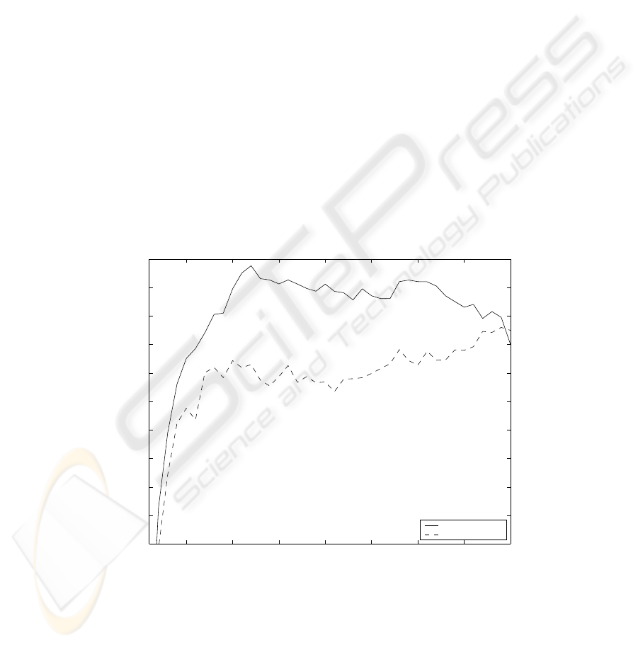
If this is done for example for one sampled ﬁfth of the waveform data using

a 1NN classiﬁer, SFS and LOOCV, the solid line in Fig. 1 can be obtained. It

appears that the optimal number of features is 12. Moreover, the peaking phe-

nomenon seems evident, suggesting that feature selection is useful in ﬁghting the

curse of dimensionality because several unnecessary and even harmful features

can be excluded. By choosing the suggested feature subset of size 12 instead of

the full set of all the 40 features, one can increase the estimated classiﬁcation

accuracy from about 74% to over 79%.

What is wrong here is that the accuracy estimates that are used to plot the

solid line are the same estimates as those that were used to guide the search

algorithm to the most beneﬁcial parts of the feature subset space. Thus, these

estimates are prone to overﬁtting, and the eﬀect of this fact will be shown in the

following.

3.2 Correct Method

If no extra data is available for independent testing, the best set found in the

previous section, that with the highest cross-validation estimate and, in case of

a draw, the smallest number of features, seems to be the most obvious guess

179

for the best feature subset. In the following, this subset is referred to as the

apparently best subset. In Fig. 1, the apparently best subset would be the one

found by the search process that has exactly 12 features.

If a proper comparison is to be made, the potentially overﬁtted results found

by the search algorithm during the search should not be used to compare the

apparently best subset and the full set. Instead, independent test data not shown

during the search has to be used. When 1NN classiﬁers are constructed using

the feature subsets found, and the remaining four ﬁfths of the waveform data are

then classiﬁed, the dashed line in Fig. 1 is obtained. It is now easy to see that

the peaking phenomenon applies only to the LOOCV estimates found during

the search, not to the accuracy obtained with the independent test data. In

fact, when comparing the apparently best subset to the full set, instead of the

increase of more than ﬁve percentage points mentioned in Sect. 3.1, a decrease

of 2.4 points is observed here.

The apparently best feature subset may seem to be very useful compared to

the full set when the evaluation scores found during the search are used in making

the comparison, but the situation can change remarkably when independent test

data is used. Why this discrepancy takes place can be easily understoo d by

recalling that there is only one candidate for the full feature set with D features,

but





candidates for subsets of size d. If, for example, D = 40 and d = 20, it

5 10 15 20 25 30 35 40

Number of features

Estimated classification accuracy (%)

LOOCV

independent test

Fig. 1. 1NN classiﬁcation accuracies for the feature subsets of the waveform dataset

found by SFS, as estimated with LOOCV during the search (solid line) and calculated

for independent test data not seen during the search (dashed line).

180

Table 2. The results for the waveform dataset with SFS. The ﬁrst column indicates

the fraction of the set used during the search that is actually used. The second and the

sixth columns denote the classiﬁcation and the CV method (LOO is LOOCV, 5CV is

ﬁvefold CV). The third and the seventh columns (d/D) show in percentage the average

size of the apparently best subset as compared to the full set. Further, the fourth and

the eighth columns (∆

) display the increase in estimated classiﬁcation accuracy due

to choosing the apparently best subset instead of the full set, as measured by the CV

estimate. Finally, the ﬁfth and the ninth columns (∆

) show the actual increase as

measured by classifying the held out test data. One standard deviation based on the

ten diﬀerent runs is shown for each value.

size method d/D (%) ∆

(%) ∆

(%) method d/D (%) ∆

(%) ∆

(%)

1/16 1NN/LOO 38 ± 11 22 ± 5 −3 ± 4 C4.5/5CV 29 ± 19 19 ± 7 −3 ± 5

1/8 51 ± 16 15 ± 5 −3 ± 2 23 ± 16 16 ± 4 2 ± 2

1/4 52 ± 16 12 ± 4 −0 ± 2 33 ± 11 10 ± 2 −0 ± 3

1/2 58 ± 13 8 ± 3 1 ± 1 44 ± 20 6 ± 2 0 ± 1

1/1 49 ± 17 5 ± 1 1 ± 2 30 ± 11 5 ± 1 0 ± 2

1/16 1NN/5CV 40 ± 1 7 20 ± 7 −2 ± 4 MLP/5CV 23 ± 11 34 ± 5 17 ± 7

1/8 50 ± 16 16 ± 5 −2 ± 3 24 ± 7 31 ± 5 18 ± 5

1/4 51 ± 16 11 ± 3 0 ± 2 22 ± 6 29 ± 4 18 ± 3

1/2 52 ± 10 8 ± 3 1 ± 1 30 ± 9 25 ± 3 19 ± 2

1/1 55 ± 12 5 ± 1 2 ± 0 39 ± 7 16 ± 2 10 ± 2

is not hard to believe that one can ﬁnd overﬁtted results amongst the more than

candidate subsets, those that would be evaluated by an exhaustive search.

This means that the results found during the search process are not only

overﬁtted, but they are more overﬁtted for some feature subset sizes than for

some others. This is because the selection of a feature subset for each size is a

model selection process, and there are simply more candidate models the closer

we are to the half of the size of the full feature set. On the other hand, the SFS

algorithm evaluates more candidates for the smaller sizes, which may result in

ﬁnding the apparently best subset size to be somewhere between the empty set

and half the full set. However, it seems that if the data is actually so diﬃcult

that the small feature subsets will not do, then the apparently best subset can

also be larger than half the full set.

3.3 More Results

We have seen that the apparently best subset can be superior to the full set when

the comparison is done using the evaluation scores found during the search, but

also that it may turn out that this is not the case when new tests are made with

previously unseen test data. Some further results are now examined in order to

assess the generality of this observation.

Table 2 shows more results for the waveform dataset. Diﬀerent kinds of classi-

ﬁcation methods are used, and all the runs are repeated for ten times — starting

with resampling the set used during the search — in order to obtain estimates for

the variance of the results. Moreover, the eﬀect of the amount of data available

during the search is visible.

The following facts can b e observed based on the table:

181

1. While non-negative by deﬁnition, ∆

is always positive and often quite

large. This means that the apparently best subset looks always better and

usually much better than the full set when the CV scores found during the

search are used for the comparison. In other words, the peaking phenomenon

is present, like in the solid curve of Fig. 1.

2. On the other hand, ∆

is pretty small — even negative — except for the

MLP classiﬁer. Therefore, the apparently best subset is not much better and

can be even worse than the full set when the comparison is performed using

independent test data. This means that usually there is hardly any peaking

with respect to the size of the feature subset when new samples are classiﬁed

— instead, the curve looks more like the dashed one in Fig. 1. Or if there

is a peak, it is not located at the same subset size as the apparently best

subset, and we actually have no means of identifying the peak unless we have

independent test data.

3. Further, ∆

is typically much greater than ∆

. This means that there is

lots of overﬁtting: the apparently best subset appears, when compared to

the full set, to be much better than it is in reality.

4. The diﬀerence between ∆

and ∆

, i.e. the amount of overﬁtting, decreases

when the size of the dataset available during the search (column “size” of the

table) increases. This is of course an expected result.

On the other hand, Table 3 shows similar results for all the datasets when

SFS is used. The dependency of the results on the amount of data available

during the search is however largely omitted for the sake of brevity. Still, ﬁgures

are shown both for 25% and 100% of the full set.

The four observations made based on Table 2 are valid also for the results in

Table 3. In addition, it is often the case that the size of the apparently best subset

divided by the size of the full set, the ratio d/D, increases when the amount of

data available increases. This is likely b ecause learning the dataset gets more

diﬃcult when the numb er of samples to learn increases, and more features are

needed to create classiﬁers that appear accurate.

Another interesting fact is that the only case where feature selection clearly

seems to help the 1NN classiﬁer, which does not even have any embedded feature

selection mechanism, is the spambase dataset. However, this is mostly due to

one feature having a much broader range of values than the others. When the

variables are normalized to unit variance as a preprocessing step, the outcome

changes remarkably (record spambase/std in Table 3).

Further, Table 4 shows the results for some of the smaller datasets with the

SFFS algorithm. Represented this way, the results do not seem to diﬀer remark-

ably from those for SFS. However, an examination of ﬁgures like Fig. 1 reveals

(not shown) that the subsets found by SFFS are typically more consistently

overﬁtted, i.e. that there is often a large numb er of subsets that are estimated to

yield a classiﬁcation accuracy equal or at least close to that obtained with the

apparently best subset, whereas for SFS the apparently best subset is typically

b etter in terms of estimated accuracy than (almost) all the other subsets.

182

Table 3. The results with SFS for all the datasets. For each method there are two

rows. On the ﬁrst row, the size of the dataset used during the search is one fourth of

the full set, whereas on the second row the full set is used (the size of which is shown in

column m of Table 1). Thus, the ﬁrst row corresponds to the third and the eighth row

of Table 2, and the second row corresponds to the ﬁfth and the tenth row. Otherwise,

the explanations for the columns equal those for Table 2.

dataset method d/D ∆

∆

method d/D ∆

∆

dermatology 1NN/LOO 30 ± 17 8 ± 7 −2 ± 4 C4.5/5CV 21 ± 11 5 ± 4 1 ± 3

59 ± 27 2 ± 1 1 ± 1 38 ± 13 2 ± 1 −1 ± 2

1NN/5CV 24 ± 6 5 ± 2 −3 ± 3 MLP/5CV 35 ± 17 20 ± 6 7 ± 4

48 ± 17 3 ± 1 −1 ± 1 54 ± 15 4 ± 2 −0 ± 2

ionosphere 1NN/LOO 18 ± 12 17 ± 6 1 ± 5 C4.5/5CV 40 ± 19 11 ± 4 1 ± 4

21 ± 10 14 ± 2 2 ± 3 30 ± 20 6 ± 2 −0 ± 2

1NN/5CV 20 ± 12 13 ± 5 0 ± 2 MLP/5CV 28 ± 15 14 ± 7 −1 ± 4

27 ± 15 10 ± 2 3 ± 2 24 ± 18 9 ± 3 4 ± 4

optdigits.tra 1NN/LOO 75 ± 17 4 ± 2 −1 ± 1 C4.5/5CV 47 ± 21 9 ± 3 −0 ± 7

72 ± 15 1 ± 0 −1 ± 0 63 ± 16 4 ± 1 −0 ± 2

1NN/5CV 64 ± 13 5 ± 1 −1 ± 1 MLP/5CV 41 ± 10 24 ± 8 16 ± 15

67 ± 12 1 ± 1 −1 ± 0 55 ± 16 8 ± 2 1 ± 3

sonar 1NN/LOO 20 ± 17 27 ± 9 −2 ± 10 C4.5/5CV 22 ± 27 25 ± 13 1 ± 4

55 ± 7 13 ± 4 2 ± 5 30 ± 23 17 ± 4 0 ± 7

1NN/5CV 21 ± 26 32 ± 8 −2 ± 7 MLP/5CV 17 ± 20 23 ± 11 −3 ± 4

35 ± 17 14 ± 3 −2 ± 6 32 ± 13 14 ± 3 −1 ± 4

spambase 1NN/LOO 37 ± 10 26 ± 4 18 ± 2 C4.5/5CV 41 ± 15 6 ± 2 −1 ± 2

49 ± 13 18 ± 2 14 ± 1 54 ± 19 3 ± 1 0 ± 1

1NN/5CV 37 ± 13 26 ± 3 18 ± 1 MLP/5CV 29 ± 12 10 ± 2 1 ± 2

44 ± 15 18 ± 2 14 ± 1 47 ± 12 3 ± 1 0 ± 1

spambase/std 1NN/LOO 37 ± 22 12 ± 3 2 ± 2 C4.5/5CV 34 ± 15 6 ± 2 −0 ± 2

42 ± 10 6 ± 1 3 ± 1 52 ± 20 3 ± 1 0 ± 1

1NN/5CV 30 ± 10 11 ± 4 3 ± 3 MLP/5CV 29 ± 12 9 ± 3 2 ± 2

43 ± 14 5 ± 1 2 ± 2 46 ± 13 3 ± 1 −0 ± 1

spectf 1NN/LOO 21 ± 10 30 ± 11 1 ± 5 C4.5/5CV 20 ± 17 19 ± 6 2 ± 6

37 ± 15 14 ± 3 1 ± 4 39 ± 24 10 ± 3 −2 ± 3

1NN/5CV 20 ± 8 25 ± 6 0 ± 5 MLP/5CV 9 ± 3 18 ± 5 −3 ± 8

34 ± 15 13 ± 4 1 ± 3 9 ± 3 10 ± 2 2 ± 4

tic-tac-toe 1NN/LOO 90 ± 21 1 ± 2 −3 ± 7 C4.5/5CV 69 ± 24 5 ± 3 −1 ± 4

100 ± 0 0 ± 0 0 ± 0 99 ± 4 0 ± 0 −0 ± 0

1NN/5CV 94 ± 6 1 ± 1 −2 ± 3 MLP/5CV 84 ± 15 2 ± 2 −4 ± 4

100 ± 0 0 ± 0 0 ± 0 100 ± 0 0 ± 0 0 ± 0

waveform 1NN/LOO 52 ± 16 12 ± 4 −0 ± 2 C4.5/5CV 33 ± 11 10 ± 2 −0 ± 3

49 ± 17 5 ± 1 1 ± 2 30 ± 11 5 ± 1 0 ± 2

1NN/5CV 51 ± 16 11 ± 3 0 ± 2 MLP/5CV 22 ± 6 29 ± 4 18 ± 3

55 ± 12 5 ± 1 2 ± 0 39 ± 7 16 ± 2 10 ± 2

wdbc 1NN/LOO 12 ± 13 9 ± 5 −2 ± 4 C4.5/5CV 14 ± 8 4 ± 3 0 ± 1

51 ± 34 3 ± 2 0 ± 2 38 ± 18 4 ± 1 1 ± 1

1NN/5CV 17 ± 14 8 ± 5 −0 ± 2 MLP/5CV 22 ± 15 36 ± 1 30 ± 2

34 ± 10 4 ± 1 −1 ± 2 29 ± 12 34 ± 3 33 ± 2

wpbc 1NN/LOO 33 ± 25 29 ± 16 1 ± 5 C4.5/5CV 16 ± 17 23 ± 9 2 ± 4

46 ± 30 15 ± 7 −5 ± 4 31 ± 18 12 ± 4 2 ± 9

1NN/5CV 22 ± 20 23 ± 12 −1 ± 7 MLP/5CV 10 ± 9 11 ± 6 −14 ± 8

31 ± 24 14 ± 4 −4 ± 5 12 ± 12 2 ± 2 −4 ± 5

183

Table 4. Like Table 3, but for SFFS and only a few datasets.

dataset method d/D ∆

∆

method d/D ∆

∆

dermatology 1NN/LOO 25 ± 11 8 ± 5 −6 ± 3 C4.5/5CV 29 ± 25 10 ± 5 1 ± 2

43 ± 12 3 ± 1 −2 ± 1 44 ± 22 3 ± 1 −0 ± 2

1NN/5CV 35 ± 26 7 ± 4 −4 ± 4 MLP/5CV 39 ± 17 21 ± 4 8 ± 6

56 ± 19 4 ± 1 −1 ± 2 48 ± 12 5 ± 1 1 ± 3

ionosphere 1NN/LOO 17 ± 9 22 ± 10 1 ± 5 C4.5/5CV 34 ± 24 10 ± 6 −2 ± 4

20 ± 6 15 ± 3 1 ± 3 45 ± 18 7 ± 3 1 ± 2

1NN/5CV 23 ± 16 17 ± 7 1 ± 5 MLP/5CV 28 ± 22 13 ± 6 0 ± 5

22 ± 9 11 ± 1 1 ± 3 25 ± 15 9 ± 1 2 ± 3

sonar 1NN/LOO 8 ± 3 31 ± 14 3 ± 4 C4.5/5CV 22 ± 23 29 ± 9 −0 ± 5

24 ± 6 16 ± 3 −1 ± 4 29 ± 20 15 ± 5 1 ± 9

1NN/5CV 23 ± 18 26 ± 11 1 ± 6 MLP/5CV 25 ± 21 23 ± 8 −5 ± 9

40 ± 16 14 ± 4 1 ± 6 33 ± 20 12 ± 3 −3 ± 6

spectf 1NN/LOO 26 ± 13 33 ± 8 4 ± 6 C4.5/5CV 18 ± 15 18 ± 8 2 ± 4

45 ± 14 16 ± 3 2 ± 4 48 ± 23 9 ± 2 −1 ± 4

1NN/5CV 23 ± 12 28 ± 5 3 ± 5 MLP/5CV 9 ± 3 18 ± 4 −2 ± 4

32 ± 15 13 ± 4 0 ± 4 12 ± 3 12 ± 3 2 ± 4

The datasets and the methods used here were chosen rather arbitrarily, which

suggests that some generality of the results can be expected. Still, there are

probably many examples where the results would look completely diﬀerent —

for instance, there can be datasets that are comprehensive enough that there is

no signiﬁcant overﬁtting.

4 Conclusions

The experimental results reported in this paper suggest that the best cross-

validation score found during the search is often obtained with a feature subset

that is much smaller than the full set, and the diﬀerence between the scores for

this apparently best feature subset and the full set of all the candidate features

is often signiﬁcant. Thus, it is possible to come up with a hasty conclusion that

removing some of the features increases the classiﬁcation score.

However, from the fact that the CV scores found during the search are un-

equally biased for diﬀerent subset sizes, it follows that the optimal subset size

for independent test data is often not the same as or even close to that of the

apparently best subset. More importantly, the apparently best subset, which

often seems to be superior over the full set when the comparison is based on

the estimates found during the search, may turn out to be even worse when

classifying new data. It appears that in many cases the peaking phenomenon is

not due to the classiﬁer being overwhelmed by the curse of dimensionality (any

more than a feature selection algorithm is), but rather an artifact solely caused

by the overﬁtting in the search process. Therefore, the results suggest that the

estimates found during the search should not be used when determining the op-

timal number of features to use. Instead, an independent test set — or, if there

is time, an outer loop of cross-validation — is needed.

184

References

[1] I. Guyon and A. Elisseeﬀ. An introduction to variable and feature selection.

J. Mach. Learn. Res., 3:1157–1182, 2003.

[2] M. Kudo and J. Sklansky. Comparison of algorithms that select features

for pattern classiﬁers. Pattern Recognition, 33(1):25–41, 2000.

[3] M. Egmont-Petersen, W.R.M. Dassen, and J.H.C. Reiber. Sequential se-

lection of discrete features for neural networks — a Bayesian approach to

building a cascade. Patt. Recog. Lett., 20(11–13):1439–1448, 1999.

[4] P. Pudil, J. Novoviˇcov´a, and J. Kittler. Floating search methods in feature

selection. Patt. Recog. Lett., 15(11):1119–1125, 1994.

[5] R. Kohavi and G. John. Wrappers for feature subset selection. Artiﬁcial

Intelligence, 97(1–2):273–324, 1997.

[6] D. Charlet and D. Jouvet. Optimizing feature set for speaker veriﬁcation.

Patt. Recog. Lett., 18(9):873–879, 1997.

[7] P. Somol and P. Pudil. Oscillating search algorithms for feature selection.

In Proc. ICPR’2000, pages 406–409, Barcelona, Spain, 2000.

[8] R. Bellman. Adaptive Control Processes: A Guided Tour. Princeton Uni-

versity Press, 1961.

[9] P.A. Devijver and J. Kittler. Pattern Recognition: A Statistical Approach.

Prentice–Hall International, 1982.

[10] G.V. Trunk. A problem of dimensionality: A simple example. IEEE Trans.

Pattern Anal. Mach. Intell., 1(3):306–307, 1979.

[11] A.W. Whitney. A direct method of nonparametric measurement selection.

IEEE Trans. Computers, 20(9):1100–1103, 1971.

[12] P. Somol, P. Pudil, J. Novoviˇcov´a, and P. Pacl´ık. Adaptive ﬂoating search

methods in feature selection. Patt. Recog. Lett., 20(11–13):1157–1163, 1999.

[13] J.R. Quinlan. C4.5: Programs for Machine Learning. Morgan Kaufmann,

1993.

[14] C.M. Bishop. Neural Networks for Pattern Recognition. Oxford University

Press, 1995.

[15] M. Riedmiller and H. Braun. A direct adaptive method for faster backprop-

agation learning: The RPROP algorithm. In Proc. ICNN93, pages 586–591,

San Francisco, CA, USA, 1993.

[16] G.H. John, R. Kohavi, and K. Pﬂeger. Irrelevant features and the subset

selection problem. In Proc. ICML-94, pages 121–129, New Brunswick, NJ,

USA, 1994.

[17] P. Perner and C. Apt´e. Empirical evaluation of feature subset selection

based on a real world data set. In Proc. PKDD-2000 (LNAI 1910), pages

575–580, Lyon, France, 2000.

[18] A.F. Frangi, M. Egmont-Petersen, W.J. Niessen, J.H.C. Reiber, and M.A.

Viergever. Bone tumor segmentation from MR perfusion images with neural

networks using multi-scale pharmacokinetic features. Image and Vision

Computing, 19(9–10):679–690, 2001.

185