Neural Network Learning:
Testing Bounds on Sample Complexity
Joaquim Marques de Sá
1
, Fernando Sereno
2
, Luís Alexandre
3
INEB – Instituto de Engenharia Biomédica
1
Faculdade de Engenharia da Universidade do Porto/DEEC, Rua Dr. Roberto Frias,
4200-465 Porto, Portugal
2
Escola Superior de Educação, Rua Dr Roberto Frias,
4200-465 Porto, Portugal
3
Universidade da Beira Interior, Dep. Informática, Rua Marquês de Ávila e Bolama
6201-001 Covilhã, Portugal
Abstract. Several authors have theoretically determined distribution-free bounds
on sample complexity. Formulas based on several learning paradigms have been
presented. However, little is known on how these formulas perform and com-
pare with each other in practice. To our knowledge, controlled experimental re-
sults using these formulas, and comparing of their behavior, have not so far been
presented. The present paper represents a contribution to filling up this gap,
providing experimentally controlled results on how simple perceptrons trained
by gradient descent or by the support vector approach comply with these
bounds in practice.
1 Introduction
Sample complexity formulas based on statistical learning theory and the probably
approximately correct (PAC) learning paradigm can be found in [2], [3], [4]. These for-
mulas assume a worst-case setting of the learning task. Other authors [6], on the con-
trary, presented a formula adequate to an average-learning setting. We are interested
in assessing the quality of these formulas when using supervised classification with
neural networks, based on the empirical error minimization (ERM) principle.
We thus assume that our NN represents a mapping φ: X → T of an object space, X
(X⊆ℜ
d
), into a target space T. For simplicity reasons, we only consider dichotomic
decisions with T = {0, 1}. We denote by φ(x,w) the NN output using some weight
vector w∈W, of a weight vector space W.
The NN learning task consists of the minimization of a risk functional:
∫
∈= WwzdFwzQwR ),(),()( with Q(z, w) =



≠
=
),(1
),(0
wxt
wxt
φ
φ
Marques de Sá J., Sereno F. and Alexandre L. (2004).
Neural Network Learning: Testing Bounds on Sample Complexity.
In Proceedings of the 4th International Workshop on Pattern Recognition in Information Systems, pages 196-201
DOI: 10.5220/0002653301960201
Copyright
c
 SciTePress

for the dichotomic data classification task, where z = (x,t) are data pairs and F(z) is the
data distribution. R(w) is then the NN probability of error, P
e
(w).
In practice, the NN is designed so to minimize the empirical error, i.e., based on a
training set D
n
= {z
i
= (x
i
, t
i
): x
i
∈X, t
i
∈T, i = 1,2,…,n}, we pick up the mapping (by suit-
able NN weight adjustment) that minimizes
∑
=
=
n
i
i
wzQ
n
wR
1
emp
),(
1
)( .
The minimum empirical risk occurs for a weight vector w
n
. )(
emp n
wR is then the resub-
stitution estimate of the probability of error,
e
P
ˆ
, of the NN classifier.
Statistical Learning Theory [9] shows that the necessary and sufficient condition
for the consistency of the ERM principle
,
, independently of the probability distribution
(independently of the problem to be solved), is:
0
)(
lim =
∞→
n
nG
n
where G(n), called growth function, can be shown to either satisfy
G(n) = n ln2 if n ≤ h
or to be bounded by:
( )






+≤





≤
∑
=
h
n
hnG
h
i
n
i
ln1ln)(
0
if n > h.
The parameter h, called the Vapnik-Chervonenkis dimension (or VC-dimension for
short) is the maximum number of vectors z
1
,…, z
h
, which can be separated in all 2
h
pos-
sible ways using the family of functions φ(z) implemented by the neural network (shat-
tered by that family). As an example, consider a single perceptron with x ∈ ℜ
2
that
uses a step function as activation function. The perceptron implements a line in 2-
dimensional space. Therefore, the determination of h amounts to determining the
maximum cardinality of a set of points that can be separated in all 2
h
possible ways by
any line. In this simple case h = 3. For more complex situations there are no exact for-
mulas of h and one has to be content with bounding formulas.
Let C be a class of possible dichotomies of the data inputs. The neural network at-
tempts to learn a dichotomy c ∈ C using a function from a family of functions Φ im-
plemented by the neural network. Using an appropriate algorithm, the neural network
learns c ∈ C with an error probability (true error rate) ε (≡ P
e
) with confidence δ. A
theorem presented in [3] establishes the PAC-learnability
1
of the class C only if its VC
1
C is PAC-learnable by an algorithm using D
n
and Φ , if for any data distribution and ∀ ε, δ, 0 <
ε, δ < 0.5 the algorithm is able to determine a function φ ∈ Φ , such that P(P
e
(φ) ≤ ε) ≥ 1−δ, in
polynomial time in 1/ε, 1/δ, n and size(c). (See [1], [5], [7])
197

dimension, h, is finite. Moreover, it establishes the following sample complexity
bounds:
1. Upper bound: For 0 < ε < 1 and sample size at least


















=
εεδε
13
log
8
,
2
log
4
max
22
h
n
u
, (1)
any consistent algorithm is of PAC learning for C.
2. Lower bound: For 0 < ε < ½ and sample size less than
( )( )( )






+−−






−
= δδε
δε
ε
121,
1
ln
1
max hn
l
, (2)
no learning algorithm is of PAC learning for C.
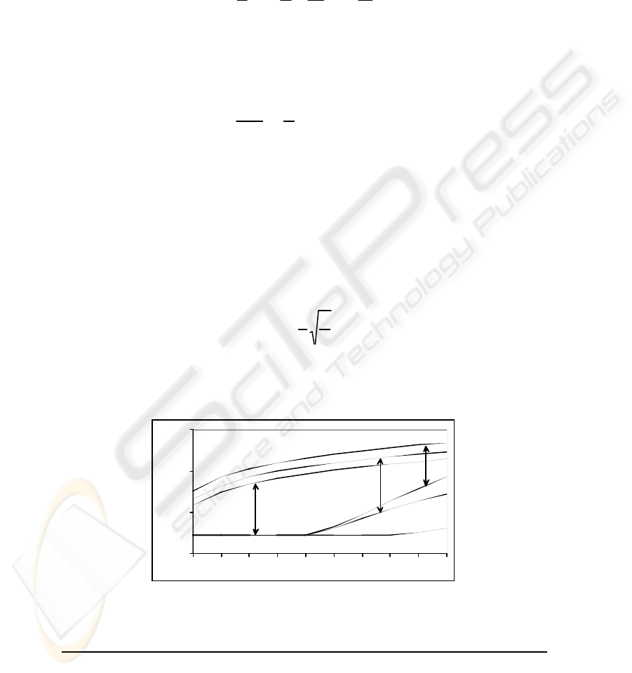
Fig. 1 illustrates these bounds for several values of the VC-dimension, h, and the
dimensionality of the input space, d, when ε = 0.05 and δ = 0.01. Notice the large gap
between lower and upper bound for small values of h.
Another approach [6] consists on bounding the Average Generalization Error
(AGE) of a learning machine, namely a MLP. This bound is obtained not in the context
of PAC theory, but from hypothesis testing inequalities. As mentioned before, it is not
a worst-case bound but an average-case bound. It has the following expression:
n
d
AGE
2
1
+<α , (3)
where α is the training error, d represents the number of adjustable parameters (for an
MLP, the number of weights) and m is the number of training points.
10
100
1000
10000
1 2 3 4 5 6 7 8 9 10
h
n
d=2
d=4
d=8
Fig. 1. Bounds of n for ε = 0.05 and δ = 0.01.
198

2 Experimental Setting
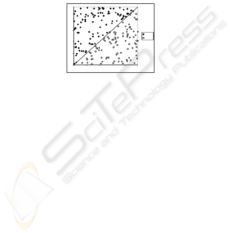
In order to test the previous bounds we must use an experimental setting where we
have perfect control on the value of h and on the value of the (true) probability of
error. These conditions are satisfied for instance for the data distribution depicted in
Fig. 2, consisting of uniformly distributed points (x
2
, x
1
) in [0, 1]
2
, linearly separated by
the x
2
= x
1
straight line.
0
0.2
0.4
0.6
0.8
1
0 0.2 0.4 0.6 0.8 1
Class 1
Class 2
Fig. 2. Example of dataset used in the experiments.
We then know that h = 3, and for any perceptron using a step function - thus, imple-
menting a straight line -, it is an easy task to determine the true error: just determine the
areas corresponding to wrongly classified points (remember that the data distribution
is uniform).
The experiments were performed as follows: a single 2-input-1-output perceptron
with step activation function was trained on a random sample D
n
⊂ [0, 1]
2
until achiev-
ing perfect separation on D
n
. This experiment was repeated a certain number of times in
order to obtain, for each n, the δ = 95% percentile of all computed probabilities of error.
Finally, using formula (2) we are able, by a table look-up procedure, to determine the
value of ε achieving the lower bound of n.
3 Results
For each value of n = 10, 20, ..., 150 we generated 25 random sets, D
n
. The (true) error
average and upper 95% percentile for the gradient descent training were determined,
as shown in Fig. 3: “Average experimental error” and “95% experimental error” curves.
Fig. 3 also shows the “95% Theoretical error” predicted by formula (2) and the AGE
bound. The theoretical error predicted by formula (1) is largely pessimistic, yielding
large values of ε (≈ 1) for the represented interval of n.
We repeated these same experiments for a support vector machine with a linear ker-
nel and the same basic architecture (SVM2:1). The results obtained are shown in Fig. 4.
199

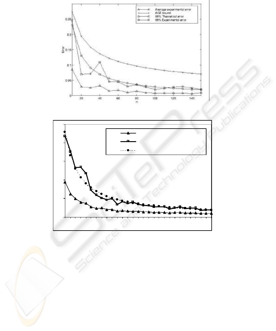
Fig. 3. Error curves for the perceptron, with the AGE bound.
0
0.05
0.1
0.15
0.2
0.25
10
20
30
40
50
60
70
80
90
100
110
120
130
140
150
Average experimental error
95% Experimental error
95% Theoretical error
Fig. 3. Error curves for the SVM2:1.
4 Discussion
The results of the previous section show that the lower bound (2) represents a tight
bound for the mentioned experiments. As a matter of fact, the “95% Experimental error”
and the “95% Theoretical error” curves are very close to each other, namely for the
larger values of n. The curves also illustrate the well-known O(1/ε) behavior for this
learning process [1]. Comparing the SVM approach with the gradient descent ap-
proach we see that the first one has smoother convergence. This is also to be expected
given the decrease of the VC-dimension for the SVM approach.
200

The AGE bound in Figure 5 is quite loose if compared with the bound from formula
(2). It also exhibits the O(1/ε) behavior of the learning process shown by the other
bound and the theoretic and measured error rates. So, although the bound from ex-
pression (2) is derived in a worst-case scenario, it is in fact tighter than the bound from
expression (3). This may not be a fair comparison since expression (2) works for a 95%
confidence interval whereas expression (3) should always be valid, hence its larger
margin from the average experimental error curve.
We are currently pursuing the experimental test of several sample complexity
bounding formulas presented in the literature, using both artificial and real datasets of
more complex nature. This raises two added difficulties: how to obtain good estimates
of the VC-dimension for spaces of higher dimensionality than ℜ
2
and using more com-
plex functions than the step function; how to obtain good estimates of the true error of
a classifier.
References
1. Anthony, M., Bartlett, P.L.: Neural Network Learning: Theoretical Foundations. Cambridge
University Press (1999)
2. Baum, E.B., Haussler, D.: What Size Net Gives Valid Generalization? Neural Computation, 1
(1989) 151-160
3. Blumer, A., Ehrenfeucht, A., Haussler, D., Warmuth, M.K.: Learnability and the Vapnik-
Chernovenkis Dimension. J Ass Comp Machinery, 36 (1989) 929-965
4. Ehrenfeucht, A., Haussler, D., Kearns, M., Valiant, L.: A General Lower Bound on the Num-
ber of Examples Needed for Learning. Information and Computation, 82 (1989) 247-261
5. Kearns, M.J., Vazirani, U.V.: An Introduction to Computational Learning Theory. The MIT
Press (1997)
6. Gu, H., Takahashi, H.: Towards more practical average bounds on supervised learning. IEEE
Trans. Neural Networks, 7 (1996) 953-968
7. Mitchell, T.M.: Machine Learning. McGraw Hill Book Co. (1997)
8. Marques-de-Sá, J.P.: Introduction to Statistical Learning Theory. Part I: Data Classification.
http://www.fe.up.pt/nnig/ (2003)
9. Vapnik, V.N.: Statistical Learning Theory. John Wiley & Sons, Inc. (1998)
201