On Designing Pattern Classifiers Using Artificially

Created Bootstrap Samples

Qun Wang and B. John Oommen

School of Computer Science Carleton University, Ottawa, Canada: K1S 5B6

Abstract: We consider the problem of building a pattern recognition classifier

using a set of training samples. Traditionally, the classifier is constructed by using

only the set

of given training samples. But the quality of the classifier is poor when

the size of the training sample is small. In this paper, we shall show that the quality

of the classifier can be improved by utilizing artificially created training samples,

where the latter are obtained by using various extensions of Efron’s bootstrap

technique. Experimental results show that classifiers which incorporate some of the

bootstrap algorithms, noticeably improve the performance of the resultant classifier.

1 Introduction

The question of how a good pattern classifier can be designed is a fundamental

problem in pattern recognition. This is, typically, achieved by using the training sample

(or set), and then designing the classifier by appropriately invoking either a parametric

or a non-parametric method. It is well known, however, that the size of the training

sample is crucial in designing a good classifier. In the case of parametric methods, if

the size of the training sample is large, the corresponding parametric estimates

converge, and so the classifier can be shown to converge to the one sought for.

Similarly, in the non-parametric case, rules like the nearest-neighbour rule have small

error only if the size of the training sample is large. Indeed, it is well known that the 1-

NN rule has an error which is less than twice the Bayes error, if the training sample

size is arbitrarily large [DHS01]. Thus, it is universally accepted that the quality of the

classifier is poor when the size of the training sample is small.

In this paper, we shall show that the quality of the classifier can be improved by

utilizing artificially created training samples, where the latter are obtained by invoking

various extensions of Efron’s bootstrap technique [Ef79]. To render this study

complete, we shall first propose various schemes by which the Bootstrap method can

be adapted to this problem, and then test them for some “benchmark” data sets.

Experimental results show that classifiers which incorporate some of the “non-local”

bootstrap algorithms, noticeably improve the performance of the resultant classifier.

This is the main thrust and contribution of this paper. We are not aware of any

other study of this nature (apart from Hamamoto et al [HUT97]), in which Bootstrap

methods are used to enhance the classifier design, when the training sample is

extremely small.

Throughout this paper we shall refer to this set in the singular, namely as the “training sample”.

Wang Q. and John Oommen B. (2004).

On Designing Pattern Classiﬁers Using Artiﬁcially Created Bootstrap Samples.

In Proceedings of the 4th International Workshop on Pattern Recognition in Information Systems, pages 159-168

DOI: 10.5220/0002653901590168

 SciTePress

1.1 Classifier Design

Despite the difference of the structures or the model of computation used, a

classifier is traditionally constructed by using only the given training sample. However,

Efron’s bootstrap technique provides a way to build a classifier by using an artificial

training sample, which, in turn, is generated from the original one. The only reported

work done in this context is by Hamamoto et al [HUT97] who first proposed bootstrap

schemes to achieve this. The details of their work (necessarily brief) constitute the

contents of Section 2. In Section 3, we introduce new pseudo-sample algorithms and

present experimental results obtained by using these schemes in Section 4.

1.2. Experimental Data Set

The data set used for all the experiments in this paper is a set of randomly

generated samples, which consists of training samples for seven classes. Each class has

a 2-dimension normal distribution with covariance matrix ∑ = I, and a training sample

size of only eight

. The expectation vectors of the seven classes are listed in TABLE 1.

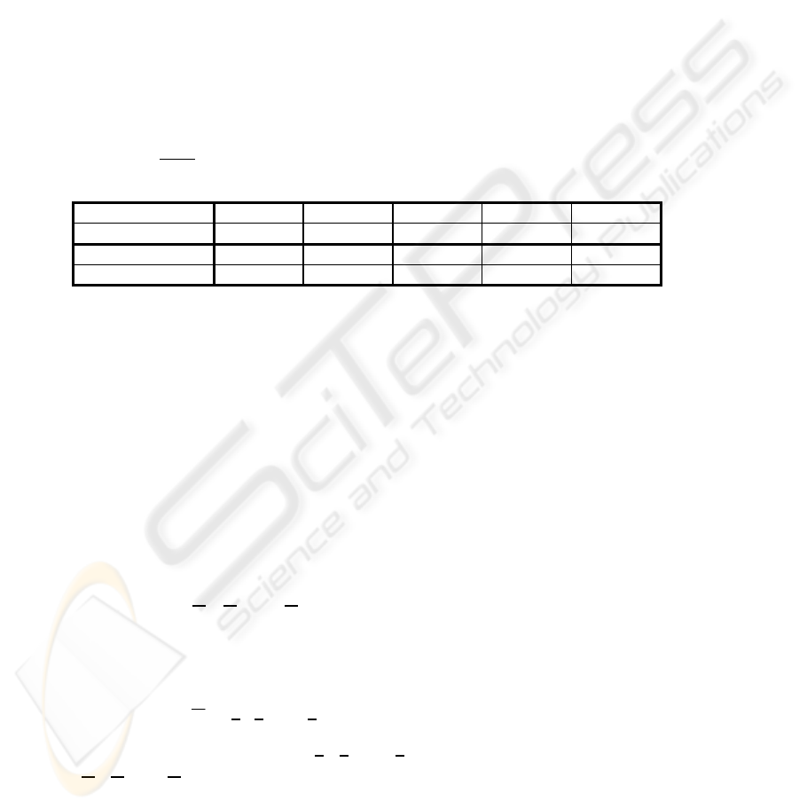
TABLE 1 : Expectations of the classes used in our experiments

CLASS A B C D E

EXPECTATION (0.0, 0.0) (0.5, 0.0) (1.1, 0.0) (1.1, 0.7) (1.1, 1.5)

CLASS F G

EXPECTATION (2.0, 1.5) (3.0, 1.5)

Only two classes are involved in each experiment: one is the class A, and the

other is selected from the rest. Hence, there are, in total, six experimental pairs of

classes, (A, B), (A, C), (A, D), (A, E), (A, F), and (A, G), where each successive pair,

tests classes which are increasingly distant from the other. With each class pair, an

experiment repeatedly does 200 trials of simulation for an algorithm. The results of the

experiments given in this paper are the average statistics from the 200 trials.

2. The Bootstrap Technique

2.1. Concept of Bootstrap

The bootstrap technique was first introduced by Efron in the late 1970’s [Ef79].

The basic strategy of bootstrap is based on resampling and simulation

Let X = {X

, X

, …, X

} be an i.i.d. d-dimension sample from an unknown

distribution F. We consider an arbitrary functional of F , θ = θ(F), which for

example, could be an expectation, a quantile, a variance, etc. The quantity θ is

estimated by a functional of the empirical distribution

F , = θ( ), where

: mass

at x

, x

, …, x

(2.1)

where n is the sample size, and {

, x

, …, x

} are the observed values of the sample

{

, X

, …, X

}. Suppose now that we can randomly generate a sample based on the

distribution,

F . Assuming the size of the sample generated is n, let this sample be :

160

= {X

, X

, …, X

(2.2)

Thus we have an empirical distribution

of the empirical distribution F ,

where,

ˆ ˆ

: mass

at x

, x

, …, x

(2.3)

and {

, x

, …, x

} are the observed values of the sample {X

, X

, …, X

and a corresponding

= θ(

) is the estimate of . θ

With the bootstrap technique, it is now possible to estimate the bias of the

estimation of as: θ

Bias = E

[ - θ ] = E

[θ( ) - θ(F)]. θ

(2.4)

Using the bootstrap empirical distribution

, the estimation of the bias (2.4) will be

Bias

= E

[

- ] = E

[θ(

) - θ( )]. θ

(2.5)

The key issue of the bootstrap technique is to obtain an empirical distribution

of the empirical distribution . It is possible to generalize the sampling scheme for

retrieving a bootstrap sample in the following way.

Let

= (P , P

,…, P

) be any probability vector on the n-dimensional

simplex

= {P

: P

≥ 0, ∑

= 1},

(2.6)

called a resampling vector [Ef82]. For a sample X

= {X

, X

, …, X

}, a re-weighted

empirical probability distribution

is defined with a resampling vector PF

: mass P on x

, i = 1, 2, …, n,

(2.7)

where {

, x

, …, x

} are the observed values of the sample {X

, X

, …, X

Generally speaking, there are three schemes that are used to retrieve an empirical

distribution

of the empirical distribution , F

Basic bootstrap

This scheme was introduced by Efron [Ef79]. In Basic bootsrap, the resampling

vector

takes the form P

= n / n, where n

is the number of x

appearing in a

bootstrap sample. This means that

follows a multinomial distribution, P

Mult(n, P

), where P

= (

,…,

) is a n-dimensional vector.

Bayesian bootstrap

This scheme was introduced by Rubin [ST95]. The scheme first generates a

sample (

, u

, …, u

n-1

) of U(0,1). It then uses the order statistics u

(0)

=0 ≤ u

(1)

≤ u

(2)

≤…

≤u

(n-1)

≤ u

(n)

=1 to define the resampling vector P

= u

(i)

- u

(i-1)

, i=1,2,…,n.

(2.8)

161

Random weighting method

This scheme was introduced by Zhen [Zh87]. It also first generates a sample (u

, …, u

) of U(0,1). Instead of using the order statistics, this scheme defines the

resampling vector

= u

/ ∑

, i=1,2,…,n.

(2.9)

2.2. SMIDAT Algorithm

The SIMDAT algorithm is due to Taylor and Thompson [TT92]. The purpose of

the SIMDAT algorithm is to provide a sampling scheme that could generate a pseudo-

data sample very close to that drawn from the kernel density function estimator of

(x) =

∑

K(x - X

, Σ

(2.10)

where the Σ

in K(•) is a locally estimated covariance matrix. Suppose {x

, x

, …, x

}

are the observed values of a sample {

, X

, …, X

}, the SIMDAT algorithm takes the

following steps,

1. Re-scale the sample data set {

, x

, …, x

} so that the marginal sample

variances in each vector component are the same;

2. For each

, find the m nearest neighbors x

(i,1)

, x

(i,2)

, …, x

(i,m)

of x

(including x

itself) and calculate the mean

of the m nearest neighbors;

3. Randomly select a sample data

from {x

, x

, …, x

};

4. Retrieve a random sample {

, u

, …, u

} from

)1(3 −m

)

and generate a pseudo-data sample using the weighted sum

=∑

(i,j)

);

Repeat Step 4 m times to get m pseudo-data samples;

Repeat Steps 3-5 N times to get a pseudo-sample of size m×N.

3 Pseudo-sample Classifier Design

3.1 Previous Work

As mentioned above, the question addressed here is one of generating an artificial

training sample set when applying the bootstrap technique to the problem of designing

a pattern classifier. Therefore, the schemes provided by Hamamoto et al [HUT97] are

for generating the synthetic training samples used to build the classifier.

Assume that the number of classes is c, and that {

1,i

, x

2,i

, …, x

} is the training

sample of the i

class, i = 1, 2,…, c. The steps of the algorithms given by Hamamoto et

al are described below :

Get the m nearest neighbors of each training pattern;

For class i, randomly select a training pattern x

j,i

and suppose its m nearest

neighbors are {

, y

, …, y

};

162

3. Retrieve a sample (u

, u

, …, u

) from U(0,1), and calculate the weighted

sum ∑

/ ∑

to get a artificial training pattern;

Repeat Step 2 and 3 n

times for class i;

Repeat Steps 2 to 4 for each class.

Some alternatives to this scheme were suggested by Hamamoto et al. One

alternative suggested that instead of randomly selecting a training pattern in Step 2, we

can just go though each training pattern in class i. A second alternative suggested that

is that in Step 3, we can use the mean of a basic bootstrap sample from the m nearest

neighbors of the training pattern, instead of their weighted sum.

The comparison of the above algorithms was done in the paper by Hamamoto

[HUT97] on the bases of the experiments with k-NN classifiers (k = 1, 3, 5). The

experiments were designed to inspect the performances of the above algorithms in

various situations, as well as the effect of dimensionality, training sample sizes, sizes

of the nearest neighbors, and the distributions. The main conclusions of their work are:

1) The algorithms outperform the conventional k-NN classifiers as well as the

edited 1-NN classifier.

2) The advantage of the algorithms comes from removing the outliers by

smoothing the training patterns, e.g. using local means to replace a training pattern.

3) The number of the nearest neighbors chosen has an effect on the result. An

algorithm was introduced to optimize the selection of this size.

The details of the experiments and the algorithm for optimizing the size of the

nearest neighbor set can be found in [HUT97].

3.2 Mixed-sample Classifier Design

We shall now show how we can specify alternate pseudo-classifier algorithms

that use a pseudo-training sample to increase the accuracy of the classifier. It is

generally accepted that the accuracy of a classifier increases with the cardinality of the

training sample. Consequently, we believe that using the pseudo-training sample set to

enlarge the training sample size is a good idea. The question that we face is one of

knowing how to generate suitable pseudo-training patterns, and to devise a

methodology by which we can blend them together with the original training samples

to build the classifier. Such a classifier design scheme is referred to as a Mixed-sample

classifier design because it uses the mixed training sample to construct the classifier.

Generally, this kind of algorithm will build a classifier in two steps: first, it will

generate a pseudo-training sample set; then it will build a classifier with all the training

patterns using both the original, and the pseudo-training samples.

The second step will be executed based on the classifier selected. This can

involve any standard classifier design algorithm based on the given training patterns.

We will thus focus on how to carry out the first step. Earlier, we presented algorithms

to generate the pseudo-training sample. We shall now modify the existing algorithms

and make them suitable for the purposes of the classifier design.

Assume that there are c classes and that {

1,i

, x

2,i

, …, x

} is the training sample

of the i

class, i = 1, 2,…, c. Below is a description of a typical algorithm for

generating a pseudo-training sample for the classifier design.

Get the m nearest neighbors of each training pattern;

For class i, randomly select a training pattern x

j,i

and suppose its m nearest

163

neighbors are {y

, y

, …, y

};

Generate a pseudo-training pattern with the m nearest neighbors {y

, y

, …,

} by applying any of the bootstrap algorithms given above, or the

SIMDAT algorithm given in Section 2.2;

Repeat Step 2 and 3 t

times for class i;

Repeat Steps 2 to 4 for each class.

As discussed

earlier, it is possible to have different weighting schemes for Step 3

of our algorithm. In our experiments, we used three different schemes: the SIMDAT

algorithm, the Bayesian bootstrap and the random weighting methods.

There are other parameters that have to be assigned before we can invoke this

algorithm. These are the number of the nearest neighbors used, and the size of the

pseudo-training sample set of each class. As expected, the pseudo-training sample size

affects the performance of the classifier. In our experiments, several pseudo-training

sample sizes were used to ascertain their effect on the performance of a classifier. The

size of the nearest neighbor set can also affect the performance of a classifier. Two

different sizes of the nearest neighbor set were used in our experiments to study their

effects.

3.3 Simulation Results

Experiments for the Mixed-sample algorithms were done with the Data Set I.

Two classes, each with a training sample of size 8, were involved in each experiment.

Sets of six different sizes, 4, 8, 12, 16, 20 and 24, were used to generate the pseudo-

training sample sets. With the size of the nearest neighbors, m = 3, three schemes

namely, the SIMDAT algorithm, the Bayesian bootstrap and the random weighting

method were used to generate the pseudo-training samples. To study the effect of the

size of the nearest neighbors, the experiments were also carried out with the size of the

nearest neighbors m = 8. Note that since the training sample size of a class is 8, a value

of m = 8 means that a pseudo-training pattern is a combination of all the patterns in the

training sample of a class. The Bayesian bootstrap and the random weighting method

were used in the experiments with a value of m = 8. To distinguish between the

Bayesian bootstrap and the random weighting method used in two different sizes of the

nearest neighbors, the previous ones are referred to as the Local-Bayesian bootstrap

and the Local-random weighting method, while the latter are simply called the

Bayesain bootstrap and the Random weighting method. After constructing a classifier

with the mixed-sample, an independent testing sample of size 1,000 for each class was

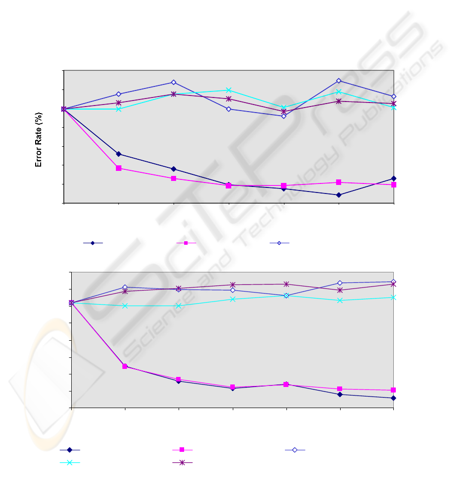
used to estimate the error rate of the 3-NN classifier. Figure 3.1 – 3.4 provide the

results of the experiments on an average of 200 trials for some of the test class-pairs.

Additional results are found in [Wu00].

The X-axis in each chart represents the pseudo-training sample size of a class, while

the Y-axis represents the error rate of the classifier estimated by the independent

testing sample. Each chart gives the results of the experiments done on one class pair.

Although, different class pairs have a different error rate; the experimental results

showed consistent tendencies, stated below.

The SIMDAT algorithm, the Local-Bayesian bootstrap and the Local-random

weighting method do not seem be advantageous. As opposed to these, the Bayesian

bootstrap and random weighting methods improve the performance of the classifier.

The effect of the pseudo-training sample increases with its size.

164

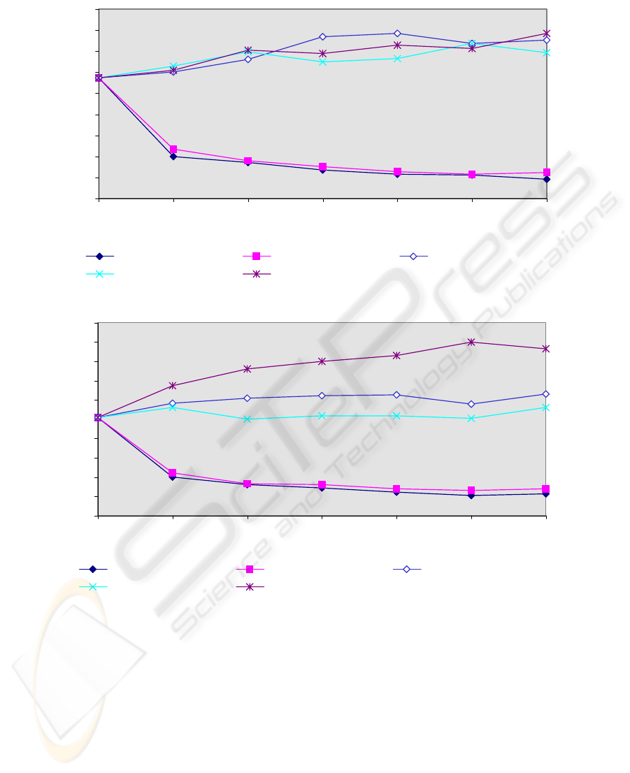
For instance, without a pseudo-training sample mixed into the original training

sample for the classifier construction, the error rate of the 3-NN classifier would be

33.37% for class pair (A, D). When the size of the pseudo-sample was increased to 16,

which is twice the size of the training sample, the classifier’s error rates increased to

34.41%, 33.82% and 34.15% for the Local-Bayesian Bootstrap, the Local-random

weighting method and the SIMDAT algorithm respectively. However, with the same

pseudo-training sample size, the error rates decreased to 31.08% and 31.14% for the

Bayesain bootstrap and the random weighting methods. This is also true for class pair

(A, E) whose experimental results can be found in [Wu00]. Without the pseudo-

training sample, the error rate of the 3-NN classifier is 23.54%. The error rates rose to

24.14%, 23.59% and 25.14% for the Local-Bayesian Bootstrap, the Local-random

weighting method and the SIMDAT algorithm respectively. At the same time, the error

rates decreased to 21.61% and 21.70% for the Bayesain bootstrap and the random

weighting method.

34.5

35.5

36.5

37.5

0 4 8 12 16 20 24

Pseudo-training Sample Size

Error Rate (%)

Bayes Bootstrap Random Weighting Local Bayes Bootstrap

Local Random Weighting SIMDAT

46.2

46.4

46.6

46.8

47.2

47.4

0 4 8 12 16 2 0 2 4

Pseudo-training Sample Size

Bayes Bootstrap

Random Weighting

Local Bayes Bootstrap

Local Random Weighting

SIM DAT

Figure 3.1 : Testing Error of the Mixed-Sample Classifier for the Class Pair (A, B)

Figure 3.2 : Testing Error of the Mixed-Sample Classifier for the Class Pair (A, C)

165

30.5

31.5

32.5

33.5

34.5

0 4 8 12 16 20 24

Pseudo-training Sample Size

Error Rate (%)

Bayes Bootstrap Random Weighting Local Bayes Bootstrap

Local Random Weighting SIMDAT

Figure 3.3 : Testing Error of the Mixed-Sample Classifier for the Class Pair (A, D)

The failure of the Local-Bayesian Bootstrap, the Local-random weighting method

and the SIMDAT algorithm indicates that the size of the nearest neighbors should not

be too small. Although, a combination of m-nearest neighbors “smooth” the training

patterns in some way, it might still be an outlier if it is the combination of m-nearest

neighbors of an outlier and the size, m, is small. The SIMDAT algorithm is the worst

one of all the schemes for class pairs (A, E), (A, F) and (A, G). The cause for this is

that the SIMDAT algorithm uses the uniform distribution

) to generate the

weighting vectors, which allows for a greater chance for an outlier point to be

Bayes Bootstrap Random Weighting Local Bayes Bootstrap

Local Random Weighting SIMDAT

22.5

23.5

24.5

25.5

Error Rate (%)

21.5

0 4 8 12 16 20 24

Pseudo-training Sample Size

Figure 3.4 : Testing Error of the Mixed-Sample Classifier for the Class Pair (A, E)

166

generated.

The algorithms of the Bayesian bootstrap and the random weighting method

performed very well as they use combinations of whole training patterns to produce the

pseudo-training sample. This confirms that the size of the nearest neighbors should not

be too small. The effect of the pseudo-training sample size is also significant. It can be

seen from Figure 3.1 – 3.4 that, for all class pairs, the larger the pseudo-training

sample’s size, the lower the error rate. The evidence show that the rate of decrease

slows down when the pseudo-training sample’s size increases. Generally, it is enough

to render the size of the pseudo-training sample to be 1.5 times (in our case m = 12) as

that of the original training sample. The results of the experiments also showed that

there is no significant performance difference between the Bayesian and the random

weighting methods.

3.4 Discussions and Conclusions

In this paper, we have discussed the problem of designing a pattern when the size

of the training sample is small. This was achieved by introducing artificially created

samples. Previously, Hamamoto et al [HUT97] constructed a classifier by weighting

the local means instead of the original training patterns. Their experiments

demonstrated that their strategy performed favorably. With the local means strategy,

they also discussed how to find the optimized size of the nearest neighbors.

What we have introduced is an alternative approach for constructing a classifier

with the so-called mixed-samples. The motivation for using the mixed-sample

classifier design was to have a larger sample size. This approach works when the

pseudo-training patterns are obtained from the weighted averages of all the original

training patterns together. However, it fails if the size of the nearest neighbors is small.

Comparing the results of the mixed-sample classifier design to the previous

results of Hamamoto et al’s work [HUT97], it may be seen that there are still

interesting problems to be discussed.

First, in terms of the mixed-sample classifier design, the designs suggested by

Hamamoto et al [HUT97] can be referred to as pseudo-training sample designs, as they

use only the pseudo-training samples – the local means – to construct a classifier. The

difference between the mixed-sample and the pseudo-training sample classifier designs

is that the latter only uses the pseudo-training sample to replace the original ones.

Second, the local means function well in the pseudo-training sample classifier

design because the local means remove the outliers by smoothing the patterns.

However, they perform badly in the mixed-sample classifier design when the size of

the nearest neighbors is small, as a bad local mean might be an extra outlier. On the

other hand, a large size of the nearest neighbors, such as the whole set of the training

sample, works well in the mixed-sample classifier design.

Third, Hamamoto et al’s work proved that a large size for the set of nearest

neighbors used does not imply that it yields the best results [HUT97]. That is why an

algorithm to optimize the size of the nearest neighbors was suggested. Hence, it

appears as if the problem of optimizing the size of the nearest neighbors for the mixed-

sample classifier design is unanswered. This could be a problem for further study.

167

Fourth, our experiments have proved that using a pseudo-training sample to

enlarge the sample size is a good strategy. As no work has been done to compare the

mixed-sample classifier design with the pseudo-training sample classifier design, it is

difficult to say which one is better.

Finally, from all of the above discussions, we confirm that the classifier design

can be improved on by using a pseudo-training sample. The problem yet to be solved is

one of knowing how to avoid the contamination of bad pseudo-patterns. There are two

possible solutions to the problem: one is to exclude the outliers from the original

training sample set before generating the pseudo-training samples. The other is to

replace the outliers in the original training sample with their local means. Although it is

believed that these two approaches are able to enhance the classifier design, they

warrant further research.

Reference

[CMN85] Chernick, M.R., Murthy, V.K. and Nealy, C.D. (1985), “Application of

bootstrap and other resampling techniques: evaluation of classifier

performance”, Pattern Recognition Letters, 3, pp.167 - 178.

[DH92] Davison, A. C. and Hall, P. (1992), “On the bias and variability of bootstrap

and cross-validation estimates of error rate in discrimination problems”,

Biometrika, 79, pp.279 - 284.

[DHS01] Duda, R.O, Hart, P. E. and Stork, D. G., (2001), Pattern Classification,

Second Edition, Wiley & Sons (2001).

[Ef79] Efron, B. (1979), “Bootstrap Method: Another Look at the Jackknife”,

Annals of Statistics, 7, pp.1 - 26.

[Ef83] Efron, B. (1983), “Estimating the error rate of a prediction rule: improvment

on cross-validation”, Journal of the American Statistical Association, 78,

pp.316 - 331.

[ET97] Efron, B. and Tibshirani, R. J. (1997), “Improvement on cross-validation: the

.632 + bootstap method”, Journal of the American Statistical Association, 92,

pp.548 - 560.

[Ha86] Hand, J.D., (1986), “Recent advances in error rate estimation”, Pattern

Recognition Letters, 4, pp.335 - 346.

[JDC87] Jain, A.K., Dubes, R.C. and Chen, C. (1987), “Bootstrap techniques for error

estimation”, IEEE Transactions on Pattern Analysis and Machine

Intelligence, PAMI-9, 628 - 633.

[TT92] Taylor, M. S. and Thompson, J. R., (1992), “A nonparametric density

estimation based resampling algorithm”, Exploring the Limits of Bootstrap,

John Wiley & Sons, Inc., pp.397 - 404.

[WO03] Wang, Q. and Oommen, B. J. (2003), “Classification Error-Rate Estimation

Using New Pseudo-Sample Bootstrap Methods”, Pattern Recognition in

Information System, PRIS-2003, Jean-Marc Ogier and Eric Trupin (Eds.), pp.

98-103.

[Wu00] Wang, Q. (2000), “Bootstrap Techniques for Statistical Pattern Recognition”,

Master Thesis, Carleton University.

[Zh87] Zhen, Z. (1987), “Random weighting methods”, Acta Math. Appl. Sinica, 10,

pp.247 - 253.

168