
Unsupervised Learning of a Finite Discrete Mixture
Model Based on the Multinomial Dirichlet Distribution:
Application to Texture Modeling
Nizar Bouguila and Djemel Ziou
D´epartement d’Informatique, Facult´e des Sciences
Universit´e de Sherbrooke
Abstract. This paper presents a new finite mixture model based on the Multino-
mial Dirichlet distribution (MDD). For the estimation of the parameters of this
mixture we propose an unsupervised algorithm based on the Maximum Likeli-
hood (ML) and Fisher scoring methods. This mixture is used to produce a new
texture model. Experimental results concern texture images summarizing and are
reported on the
Vistex
texture image database from the MIT Media Lab.
1 Introduction
Scientific pursuits and human activity in general generate data. These data may be in-
complete, redundant or erroneous. Statistical pattern recognition methods are particu-
larly useful in understanding the patterns present in such data. The finite mixture den-
sities appears as the fundamental model in areas of statistical pattern recognition. A
mixture model consists of multiple probability density function (PDFs). The PDFs are
called components densities of the mixture and are chosen to be Gaussian in the major-
ity of cases. The Gaussian mixture is not the best choice in all applications, however,
and it will fail to discover
true
structure where the partitions are clearly non-Gaussian
[14]. In [4] we have shown that the Dirichlet distribution can be a very good choice to
overcome the disadvantages of the Gaussian. In this paper, we present another distribu-
tion based in the Dirichlet and the multinomial distributions which we call the MDD
(Multinomial Dirichlet Distribution). We prove, through a novel texture model, that the
MDD is very efficient to model discrete data (vectors of counts) for them the Gaussian
is not an appropriate choice. In order to solve the problem of MDD mixture parameters
estimation, we propose an algorithm based on the Fisher scoring method and we use an
entropy-based criterion to determine the number of components.
The paper is organized as follows. The next section describes the MDD mixture in de-
tails. In section 3, we propose a method for estimating the parameters of this mixture.
In section 4, we present a way of initializing the parameters and give the complete esti-
mation algorithm. Section 5 is devoted to experimental results. We end the paper with
some concluding remarks.
Bouguila N. and Ziou D. (2004).
Unsupervised Learning of a Finite Discrete Mixture Model Based on the Multinomial Dirichlet Distribution: Application to Texture Modeling.
In Proceedings of the 4th International Workshop on Pattern Recognition in Information Systems, pages 118-127
DOI: 10.5220/0002658601180127
Copyright
c
SciTePress
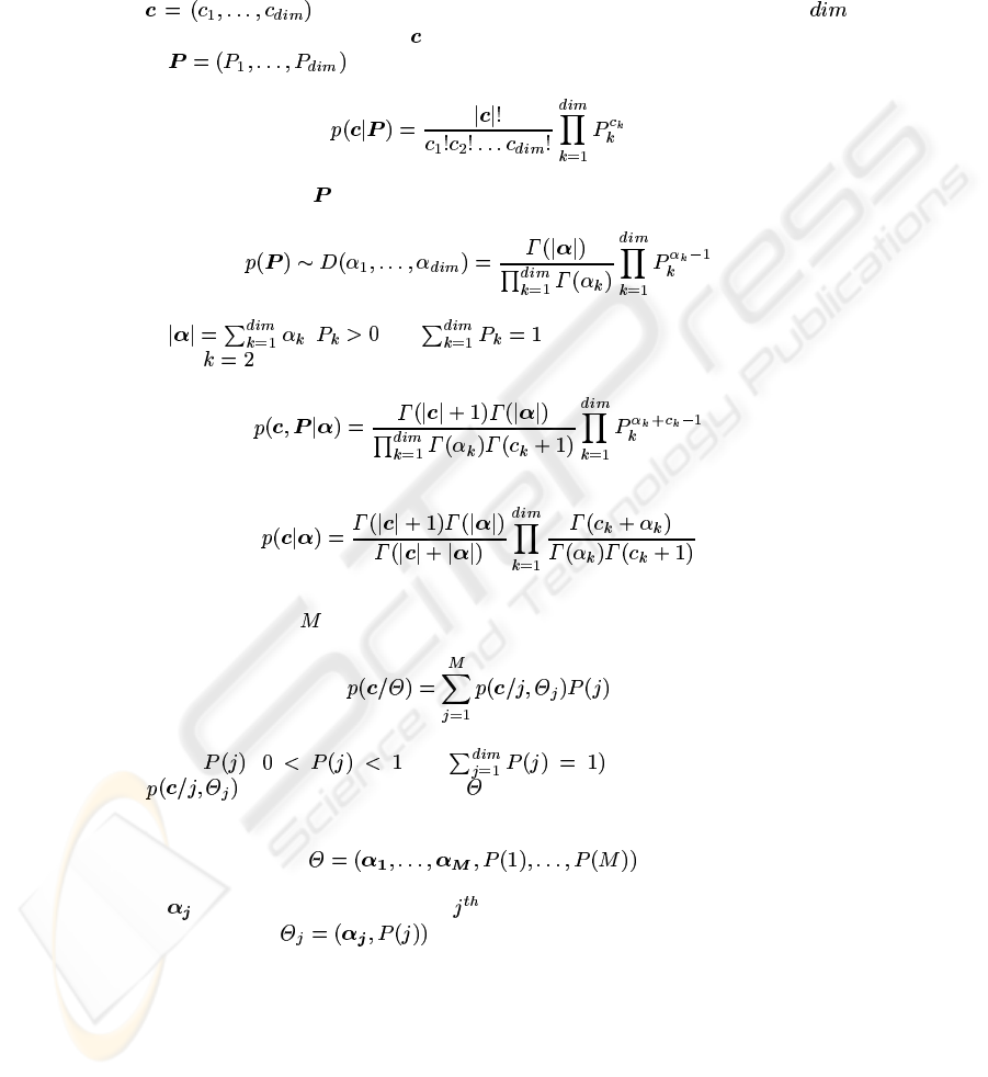
2 The Multinomial Dirichlet Mixture
Let denotes a vector of counts (ex. the frequency of a given
features in a document). The vector follows a Multinomial distribution with parameter
vector
given by:
(1)
The conjugate prior for
is the dirichlet distribution:
(2)
where
, and . The Beta distribution is the special
case when
. Given a Dirichlet prior, the joint density is:
(3)
then [4]:
(4)
We call this density the MDD (Multinomial Dirichlet Distribution).
A MDD mixture with
components is defined as :
(5)
where the
( and are the mixing proportions
and
is the MDD. The symbol refers to the entire set of parameters to be
estimated:
where is the parameter vector for the population.In the following developments,
we use the notation
forj=1...M.
3 Maximum Likelihood Estimation
The problem of estimating the parameters which determine a mixture has been the
subject of diverse studies [5]. During the last two decades, the method of maximum
likelihood (ML) has become the most common approach to this problem. Of the variety
119
of iterative methods which have been suggested as alternatives to optimize the param-
eters of a mixture, the one most widely used is Expectation Maximization (EM). EM
was originally proposed by Dempster et al. [6] for estimating the Maximum Likelihood
Estimator (MLE) of stochastic models. This algorithm gives us an iterative procedure
and the practical form is usually simple. But, it suffers from the following drawback:the
need to specify the number of components each time. In order to overcome this prob-
lem, criterion functions have been proposed, such as the Akaike Information Criterion
(AIC) [8], Minimum Description Length (MDL) [9] and Schwartz’s Bayesian Inference
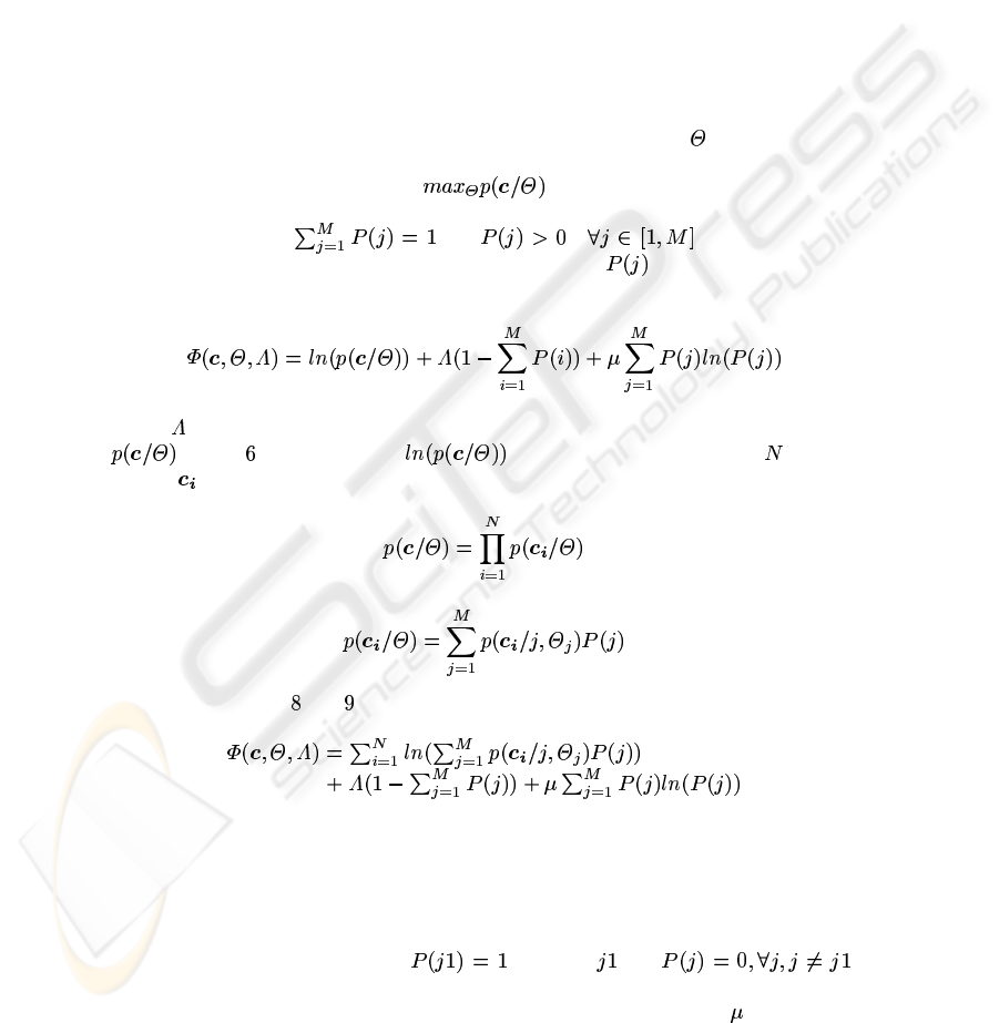
Criterion (BIC) [7]. A maximum likelihood estimate associated with a sample of obser-
vations is a choice of parameters which maximizes the probability density function of
the sample. Thus, with ML estimation, the problem of determining
becomes:
(6)
with the constraints:
and . These constraints
permit us to take into consideration
apriori
probabilities . Using Lagrange multi-
pliers, we maximize the following function:
(7)
where
is the Lagrange multiplier. For convenience, we have replaced the function
in Eq. by the function . If we assume that we have random
vectors
which are independent, we can write:
(8)
(9)
Replacing equations and , we obtain:
(10)
In order to automatically find the number of components needed to model the mixture,
we use an entropy-basedcriterionpreviously used in the case of Gaussian mixtures [10].
Thus, the first term in Eq. 10 is the log-likelihood function, and it assumes its global
maximum value when each component represents only one of the feature vectors. The
last term (entropy) reaches its maximum when all of the feature vectors are modeled
by a single component, i.e., when
for some and .
The algorithm starts with an over-specified number of components in the mixture, and
as it proceeds, components compete to model the data. The choice of
is critical to
the effective performance of the algorithm, since it specifies the tradeoff between the
120
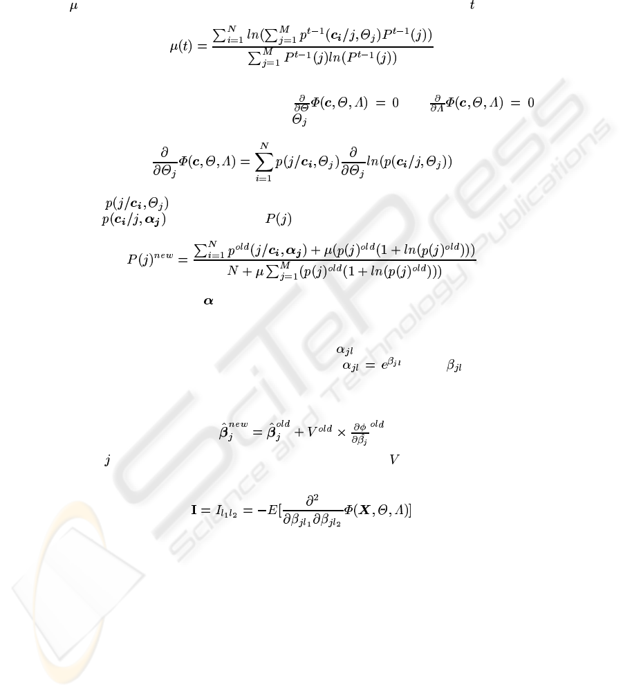
required likelihood of the data and the number of components to be found. We choose
to be the ratio of the first term to the last term in Eq. 10 of each iteration , i.e.,
(11)
We will now try to resolve this optimization problem. To do so, we must determine
the solution to the following equations:
and
Calculating the derivative with respect to :
(12)
where
is the a posterior probability.
Since
is independent of , straight forward manipulations yield:
(13)
In order to estimate the
parameters we will use Fisher’s scoring method. This ap-
proach is a variant of the Newton-Raphson method. The scoring method is based on the
first, second and mixed derivatives of the log-likelihood function. Thus, we have com-
puted these derivatives [4]. During iterations, the
can become negative. In order to
overcome this problem, we reparametrize, setting
,where is an uncon-
strained real number. Given a set of initial estimates, Fisher’s scoring method can now
be used. The iterative scheme of the Fisher method is given by the following equation
[11]:
(14)
where
is the class number.The variance-covariancematrix is obtainedas the inverse
of the Fisher’s information matrix:
(15)
An interesting geometric interpretation of this iterative scheme is given in [4]
4 Algorithm
In order to make our algorithm less sensitive to local maxima, we have used some
initialization schemes including the Fuzzy C-means [13] and the method of moments
(MM) [4]. Thus, our initialization method can be summed up as follows:
INITIALIZATION Algorithm
1. Apply the Fuzzy C-means to obtain the elements, covariance matrix and mean of
each component.
121
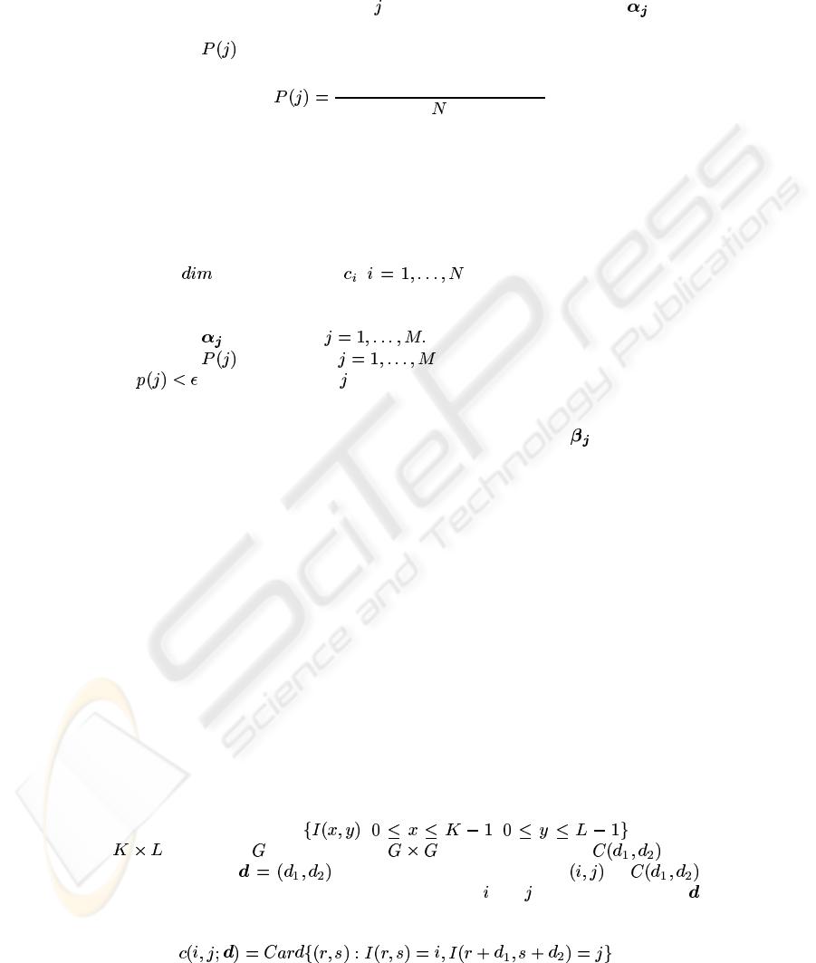
2. Apply the MM for each component to obtain the vector of parameters .
3. Assign the data to clusters, assuming that the current model is correct.
4. Update the
using this equation:
Number of elements in class j
(16)
5. If the current model and the new model are sufficiently close to each other, termi-
nate, else go to 2.
With this initialization method in hand, our algorithm for estimating a Dirichlet mixture
can be summarized as follows:
MDD MIXTURE ESTIMATION Algorithm
1. INPUT:
-dimensional data , and an over-specified number of
clusters M.
2. INITIALIZATION Algorithm.
3. Update the
using Eq. 14,
4. Update the using Eq. 13, .
5. If
discard component ,goto3.
6. If the convergence test is passed, terminate, else go to 3.
The convergence tests could involve testing the stabilization of the
or the value of
the maximum likelihood function.
5 Application: Texture Modeling
Texture analysis and modeling is an important component in image processing and is
fundamental to many applications areas including industrial automation, remote sens-
ing, and biomedical image processing. Texture is essentially a neighborhood property.
Recent work by Tuceryan and Jain provides a comprehensive survey of most existing
structural and statistical approaches to texture [1].
One of the most established method for texture modeling is the Spatial Gray Level
method which was proposed by Haralick [2]. It’s based on the estimation of the joint
probability functions of two picture elements in some given relative position (cooccur-
rence matrices). The cooccurrence matrices are mostly used as intermediate feature and
dimensionality reduction is performed in computing features of the types described in
[3]. The main drawbacks to using cooccurrence matrices is the large memory require-
ment for storing them and the difficulty to use them for statistical approaches because
of their numerical nature.
In the following, we will use
, , to denote
an
image with grey levels. The cooccurrence matrix for a
displacement vector
is defined as follows. The entry of
is the number of occurrences of the pair of gray levels and which are a distance
apart. Formally, it is given as:
(17)
122
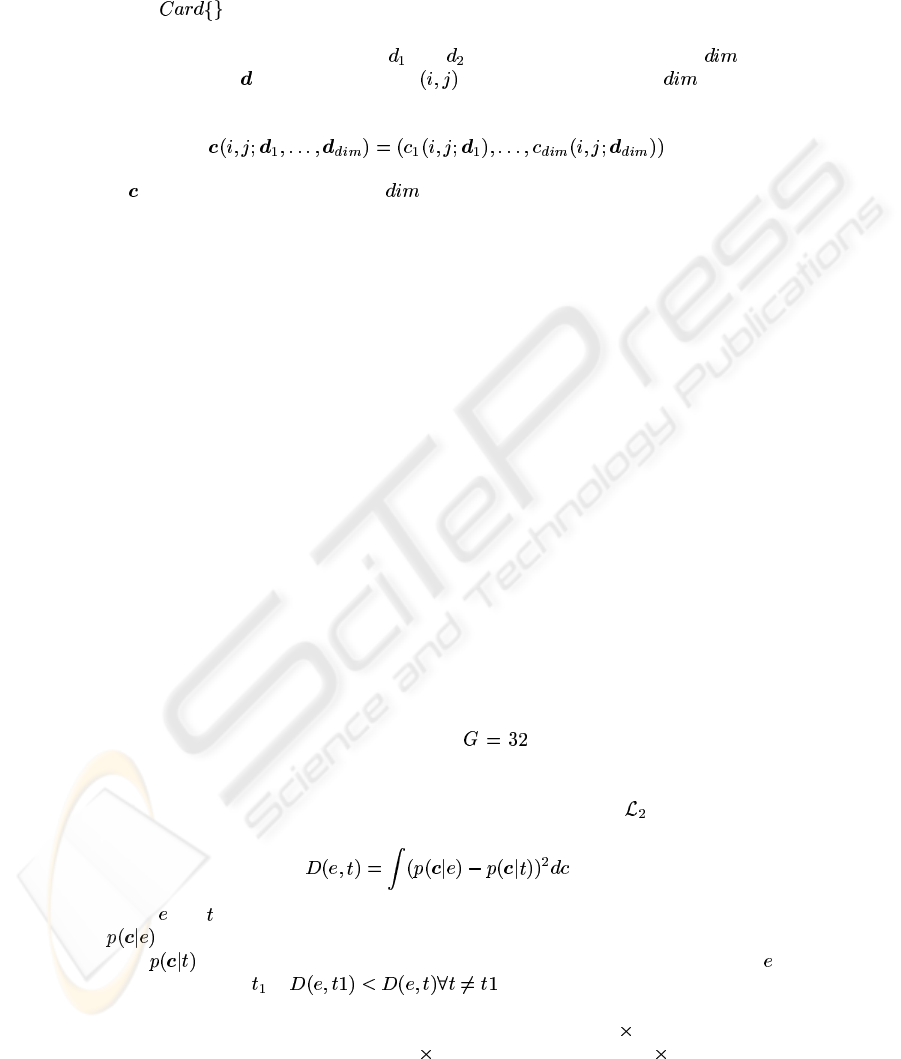
Where refers to the number of elements of a set. It’s possible to character-
ize a particular texture sample by a collection of cooccurrence matrix that have been
estimated for different displacement
and . In fact suppose that we have dis-
placement vector
, then for each entry we will have a vector of elements
given as follows:
(18)
As
is a vector of frequencies, the cooccurrence matrices can be modeled by a
mixture of MDD. With this model in hand, we use it for two experiments: texture im-
ages summarizing and retrieval.
5.1 Texture Images Summarizing
Automatic texture images summarizing is an important problem in image processing
applications. In the texture images summarizing problem, an image is known to contain
data from one of a finite number of texture classes, and it is desired to assign the im-
age to the correct class on the basis of measurements made over the entire image. This
application is very important especially in the case of content-based image retrieval.
Summarizing the database simplifies the task of retrieval by restricting the search for
similar images to a smaller domain of the database. Summarization is also very efficient
for browsing. Knowing the categories of images in a given database allows the user to
find the images he is looking for more quickly [12]. A block diagram outlining our ap-
proach to solve the texture summarizing problem is shown in Fig. 1. The inputs to the
classifier are images from a finite number of texture classes. These images are separated
into the unknownor test set of images, whose texture class is unknown, and the training
set of images, whose texture class is known. The training set is necessary to adapt the
classifier to each possible texture class before the unknown set is applied to the classi-
fier. All the input images are passed through the cooccurrence matrices computing stage
and then the mixture’s parameters estimation stage in which these cooccurrence matri-
ces are modeled as an MDD mixture (we use
). After this stage every texture
class is represented by a MDD mixture. Finally, the classification stage uses mixtures
estimated on the unknown images to determinate which texture class is present. In fact,
the estimated mixture is compared to the trained ones by using the
distance for the
densities defined by:
(19)
Where
and index respectively an MDD mixture of a texture image to be classified
(
) and an MDD mixture obtained from training and which represents a texture
class (
). Then, the classification will be performed by using this rule: the image
is assigned to class if .
For the results in this paper, we use the
Vistex
texture database obtained from the
MIT Media Lab. In our experimental framework, each of the 512
512 images from
the
Vistex
database was divided into 64 64 images. Since each 512 512 ”mother
123
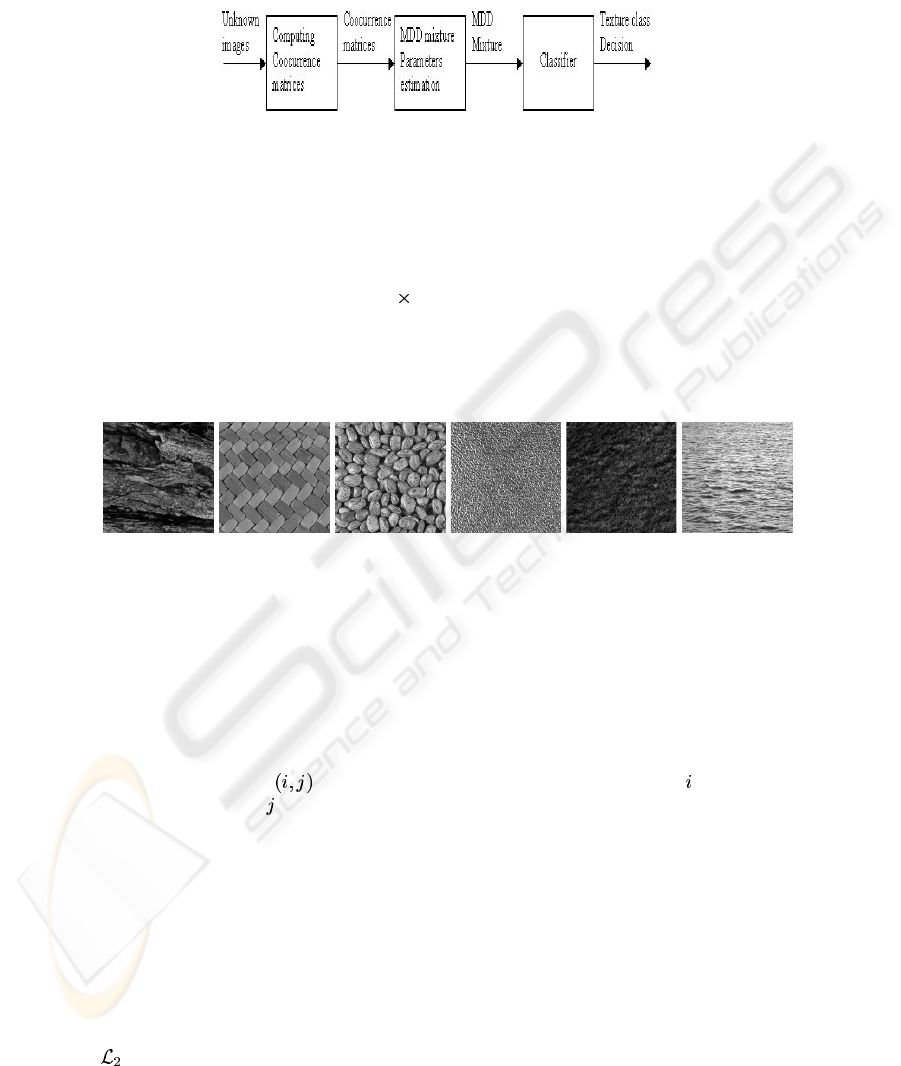
Fig.1. Block diagram of image texture summarizing application.
image” contributes 64 images to our database, ideally all the 64 images should be clas-
sified in the same class. In the experiment, six homogeneous texture groups, ”bark”,
”fabric”, ”food”, ”metal”, ”water” and ”sand” were used to create a new database. A
database with 1920 images of size 64
64 pixels was obtained. Four images from the
bark, fabric and metal texture groups were used to obtain 256 images for each of these
categories, and 6 images from the water, food and sand were used to obtain 384 images
for this category. Examples of images from each of the categories are shown in Fig. 2.
(a) (b) (c) (d) (e) (f)
Fig.2. Sample images from each group. (a) Bark, (b) Fabric, (c)Food, (d) Metal, (e) Sand, (f)
Water.
After computing the cooccurrence matrices, each category of images will be mod-
eled by a MDD mixture. Table 1 gives the parameters of these mixtures when we con-
sider 8 displacements.
The confusionmatrix of the texture images classification is given in table 2. In this con-
fusion matrix, the cell
represents the number of images from category which are
classified as category
. The number of images misclassified was: 38 images, which rep-
resents an accuracy of 98.02 percent. For comparison, we have used Gaussian mixture
instead of the MDD one. Table 3 shows the confusion matrix when Gaussian mixtures
is used (81 misclassified image, i.e an accuracy of 95.79). From the tables, we see that
the performance of the MDD mixture is better.
After the database was summarized, we conducted another experiment designed to
retrieve images similar to a query.
5.2 Texture Images Retrieval
To retrieve images that are similar to a query two-step sequence is followed. First, the
distance was used to find the two categories closest to the query by comparing
124

Category MDD Mixture parameters
Bark
class P(j)
class1 0.153 006.959 006.789 006.943 006.770 006.924 006.909 006.981 006.988
class2 0.241 011.032 012.354 011.799 011.743 011.622 012.353 011.198 011.982
class3 0.133 004.283 006.602 6.709 006.871 005.152 006.645 007.542 007.331
class4 0.201 024.685 015.902 016.022 015.908 021.489 015.920 013.616 013.620
class5 0.141 005.853 006.475 006.323 006.474 005.998 006.342 006.404 006.455
class6 0.131 005.658 005.941 006.023 005.964 005.795 006.035 006.244 006.206
Fabric
class1 0.258 025.386 022.075 023.681 022.517 026.823 025.745 025.192 024.311
class2 0.261 112.721 120.025 119.351 109.494 105.727 105.704 113.218 117.024
class3 0.266 556.039 595.921 573.386 583.624 512.379 518.183 522.132 532.666
class4 0.215 011.525 011.477 011.380 011.455 012.298 12.331 12.229 11.879
Food
class1 0.205 022.871 022.037 020.157 022.649 023.620 023.145 022.324 021.280
class2 0.165 004.914 007.579 006.025 006.969 008.663 010.282 012.798 011.390
class3 0.144 040.978 037.249 042.325 037.690 032.248 030.280 028.814 032.241
class4 0.164 004.684 007.368 005.662 006.805 008.725 010.188 012.726 011.234
class5 0.146 096.283 084.071 107.244 085.898 066.255 064.771 057.927 071.078
class6 0.176 012.889 013.675 012.205 013.282 015.050 015.165 015.388 014.079
Metal
class1 0.233 019.143 016.351 020.814 018.257 014.195 013.714 014.422 013.947
class2 0.121 006.077 005.706 006.141 006.019 005.650 005.508 005.599 005.557
class3 0.239 014.560 015.379 013.888 015.914 016.619 016.503 016.439 017.173
class4 0.242 017.159 016.779 016.589 016.944 017.009 016.151 016.517 016.376
class5 0.165 005.848 007.433 005.629 005.579 007.619 008.433 007.985 007.971
Sand
class1 0.287 007.062 008.344 007.069 007.607 008.798 008.944 009.106 008.709
class2 0.337 013.811 014.133 013.802 013.945 014.409 014.645 014.781 14.419
class3 0.376 128.296 114.760 129.365 122.650 110.878 106.602 104.713 109.643
Water
class1 0.504 846.694 832.655 853.937 857.329 797.566 804.157 805.096 822.290
class2 0.496 135.545 135.492 135.237 135.450 136.719 136.355 136.490 135.512
Table 1. Estimation of the parameters of the MDD Mixture for the different categories when we
consider 8 displacements.
the query to each representative images of the different categories. The same distance
measure was used in the second step to determine the similarity between the query and
the elements within the two closest components. The best
images were then retrieved,
where
depending on the experiment. To measure the retrieval rates, each image was
used as a query and the number of relevant images among those that were retrieved
was noted. Precision and Recall, which are the measures most commonly used by the
information retrieval community, was then computed using Eq. 20 and Eq. 21. These
measures was then averaged over all the queries.
precision
number of images retrieved and relevant
total number of retrieved images
(20)
recall
number of images retrieved and relevant
total number of relevant images
(21)
125

Bark Fabric Food Metal Sand Water
Bark 252 0 0 0 4 0
Fabric 0 250 6 0 0 0
Food 0 5 379 0 0 0
Metal 0 0 0 256 0 0
Sand 2 0 0 0 382 0
Water 1 0 0 5 2 376
Table 2. Confusion matrix for image classification by classifier based on the MDD mixture.
Bark Fabric Food Metal Sand Water
Bark 243 0 0 3 8 2
Fabric 0 240 10 0 4 2
Food 0 12 367 4 0 1
Metal 0 0 0 249 2 5
Sand 7 0 0 0 374 3
Water 4 0 0 8 6 366
Table 3. Confusion matrix for image classification by using texture features from cooccurrence
matrices and Gaussian mixture.
As each 512 512 images from the
Vistex
gives 64 images to our database, given
a query image, ideally all the 64 images should be retrieved and are considered to be
relevant. Table 4 and table 5 presents the retrieval rates in term of precision and recall
obtained when the two methods were used. The results are shown when 16, 48, 64, 80,
96 and 128 images were retrieved from the database in response to a query.
No. of retrieved images
Method
MDD Mixture
Gaussian Mixture
16 48 64 80 96
0.93 0.95 0.92 0.80 0.66
0.87 0.91 0.85 0.77 0.66
Table 4. Precision obtained for the texture database.
6Conclusion
In this paper, we have introduced a new mixture based on the Dirichlet and the multi-
nomial distributions. We estimated the parameters of this mixture using the maximum
likelihood and Fisher scoring methods. The experiments involved a new texture model
and its application to texture image databases summarizing for efficient retrieval. A
comprehensive performance evaluation of the model is given using a large number of
texture images and a comparison to other model. The MDD mixture is currently used
126

No. of retrieved images
Method
MDD Mixture
Gaussian Mixture
16 48 64 80 96
0.23 0.71 0.92 0.94 0.96
0.21 0.68 0.82 0.92 0.93
Table 5. Recall obtained for the texture database.
in a lot of other applications which involve discrete data or cooccurrence matrices such
as textmining, Webmining and E-mail segmentation.
Acknowledgment
The completion of this research was made possible thanks to Bell Canada’s support
through its Bell University Laboratories R&D program.
References
1. M. Tuceryan and A. K. Jain, Texture Analysis, The Handbook of Pattern Recognition and
Computer Vision, pp. 207-248, 1998.
2. R. M. Haralick, K. Shanmugan, and I. Dinstein Textural features for image classification,
IEEE Tr ansactions on Systems, Man and Cybernetics, vol. 8, pp. 610-621, 1973.
3. M. Unser, Sum and Difference Histograms for Texture Classification, IEEE Tr ansactions on
Pattern Recognition and Machine Intelligence, vol. 8, No. 1, pp. 118-125, 1986.
4. N. Bouguila, D. Ziou and J. Vaillancourt, Novel Mixtures Based on the Dirichlet Distribution:
Application to Data and Image Classification , IAPR International Conference on Machine
Learning and Data Mining, lNCS2734, pp. 172-181, 2003.
5. R. A. Redner and H. F. Walker, Mixture Densities, Maximum Likelihood and EM Algorithm
, SIAM Review, vol. 26, No. 2, pp. 195-239, 1984.
6. A. P. Dempster, N. M. Laird and D. B. Rubin, Maximum Likelihood from Incomplete Data
via the EM Algorithm , Journal of the Royal Statistical Society, B, vol. 39, pp. 1-38, 1977.
7. G. Schwarz, Estimating the Dimension of a Model , The Annals of Statistics, vol. 6, No. 2, pp.
461-464, 1978.
8. H. Akaike, A New Look at the Statistical Model Identification , IEEE Transactions on Auto-
matic Control, vol. AC-19, No. 6, pp. 716-723, 1974.
9. J. Rissanen, Modeling by Shortest Data Description , Biometrika, vol. 14, pp. 465-471, 1978.
10. S. Medasani and R. Krishnapuram, Categorization of Image Databases for Efficient Retrieval
Using Robust Mixture Decomposition, Computer Vision and Image Understanding, vol. 83,
pp. 216-235, 2001.
11. C. R. Rao, Advanced Statistical Methods in Biomedical Research, New York: John Wiley
and Sons, 1952
12. N. Bouguila, D. Ziou and J. Vaillancourt, Probabilistic Multimedia Summarizing Based on
the Generalized Dirichlet Mixture, Supplementary Proceedings of ICANN/ICONIP 2003,pp
150-154, 2003.
13. J. C. Bezdek, Pattern Recognition with Fuzzy Objective Function Algorithms, Plenum Press,
New York, 1981.
14. A. E. Raftery and J. D. Banfield, Model-Based Gaussian and Non-Gaussian Clustering Bio-
metrics, vol. 49, pp. 803-821, 1993.
127
