An Online Ensemble of Classifiers

S. B. Kotsiantis, P. E. Pintelas

Educational Software Development Laboratory

Department of Mathematics, University of Patras, Greece

Abstract.

Along with the explosive increase of data and information, in-

cremental learning ability has become more and more important for ma-

chine learning approaches. The online algorithms try to forget irrelevant

information instead of synthesizing all available information (as opposed

to classic batch learning algorithms). Nowadays, combining classifiers is

proposed as a new direction for the improvement of the classification ac-

curacy. However, most ensemble algorithms operate in batch mode. For

this reason, we propose an online ensemble of classifiers that combines an

incremental version of Naive Bayes, the Voted Perceptron and the Win-

now algorithms using the voting methodology. We performed a large-

scale comparison of the proposed ensemble with other state-of-the-art al-

gorithms on several datasets and we took better accuracy in most cases.

1 Introduction

Supervised learning algorithms are presented with instances, which have already been

pre-classified in some way. That is, each instance has a label, which identifies the

class to which it belongs and so this set of instances is sub-divided into classes. Su-

pervised machine learning explores algorithms that reason from the externally sup-

plied instances to produce general hypotheses, which will make predictions about

future instances.

To induce a hypothesis from a given dataset, a learning system needs to make as-

sum

ptions about the hypothesis to be learned. These assumptions are called biases. A

learning system without any assumptions cannot generate a useful hypothesis since

the number of hypotheses that are consistent with the dataset is usually huge. Since

every learning algorithm uses some biases, it behaves well in some domains where its

biases are appropriate while it performs poorly in other domains [17]. For this reason,

combining classifiers is proposed as a new direction for the improvement of the clas-

sification accuracy [3].

However, most ensemble algorithms operate in batch mode, i.e., they repeatedly

read and process the entire

training set. Typically, they require at least one pass

through the training set for every base model to be included in the ensemble. The

base model learning algorithms themselves may require several passes through the

training set to create each base model. In situations where data is being generated

continuously, storing data for batch learning is impractical, which makes using these

B. Kotsiantis S. and E. Pintelas P. (2004).

An Online Ensemble of Classiﬁers.

In Proceedings of the 4th International Workshop on Pattern Recognition in Information Systems, pages 59-68

DOI: 10.5220/0002672400590068

 SciTePress

ensemble learning algorithms impossible. These algorithms are also impractical in

situations where the training set is large enough that reading and processing it many

times would be prohibitively expensive.

Incremental learning ability is very important to machine learning approaches de-

signed for solving real-world problems due to two reasons. Firstly, it is almost impos-

sible to collect all helpful training examples before the trained system is put into use.

Therefore when new examples are fed, the learning approach should have the ability

of doing some revisions on the trained system so that unlearned knowledge encoded

in those new examples can be incorporated. Secondly, modifying a trained system

may be cheaper in time cost than building a new system from scratch, which is useful

especially in real-time applications.

We propose an ensemble that combines an incremental version of Naive Bayes, the

Voted Perceptron and the Winnow algorithms using the voting methodology. We

performed a large-scale comparison of the proposed ensemble with other state-of-the-

art algorithms on several datasets and we took better accuracy in most cases.

Section 2 introduces some basic themes about online learning, while section 3 dis-

cusses the proposed ensemble method. Experiment results and comparisons of the

proposed combining method with other learning algorithms in several datasets are

presented in section 4. Finally, we conclude in Section 5 with summary and further

research topics.

2 Online Learning

When comparing online and batch algorithms, it is worthwhile to keep in mind the

different types of setting where they may be applied. In a batch setting, an algorithm

has a fixed collection of examples in hand, and uses them to construct a hypothesis,

which is used thereafter for classification without further modification. In an online

setting, the algorithm continually modifies its hypothesis as it is being used; it repeat-

edly receives a pattern, predicts its classification, finds out the correct classification,

and possibly updates its hypothesis accordingly.

The on-line learning task is to acquire a set of concept descriptions from labelled

training data distributed over time. This type of learning is important for many appli-

cations, such as computer security, intelligent user interfaces, and market-basket

analysis. For instance, customer preferences change as new products and services

become available. Algorithms for coping with concept drift must converge quickly

and accurately to new target concepts, while being efficient in time and space.

Desirable characteristics for incremental learning systems in environments with

changing contexts are: a) the ability to detect a context change without the presenta-

tion of explicit information about the context change to the system, b) the ability to

quickly recover from a context change and adjust the hypotheses to fit the new con-

text and c) the capability to make use of previous experience in situations where old

contexts reappear.

Online learning algorithms process each training instance once "on arrival" with-

out the need for storage and reprocessing, and maintain a current hypothesis that

reflects all the training instances seen so far. Such algorithms are also useful with

very large datasets, for which the multiple passes required by most batch algorithms

are prohibitively expensive.

Some researchers have developed online algorithms for learning traditional ma-

chine learning models such as decision trees [18]. Given an existing decision tree and

a new example, this algorithm adds the example to the example sets at the appropriate

nonterminal and leaf nodes and then confirms that all the attributes at the nonterminal

nodes and the class at the leaf node are still the best.

Batch neural network learning is often performed by making multiple passes

(known in the literature as epochs) through the data with each training example proc-

essed one at a time. Thus, neural networks can be learned online by simply making

one pass through the data. However, there would clearly be some loss associated with

only making one pass through the data [15].

There is a known drawback for all these algorithms since it is very difficult to per-

form learning with several examples at once. In order to solve this problem, some

algorithms rely on windowing techniques [19] which consist in storing the n last

examples and performing a learning task whenever a new example is encountered.

The Weighted Majority (WM) algorithm [11] forms the basis of many online algo-

rithms. WM maintains a weight vector for the set of experts, and predicts the outcome

via a weighted majority vote between the experts. WM online learns this weight vec-

tor by “punishing" erroneous experts. A number of similar algorithms have been

developed such as [2].

The concept of combining classifiers is proposed as a new direction for the im-

provement of the performance of classifiers [3]. Unfortunately, in an on-line setting,

it is less clear how to apply ensemble methods directly. For instance, with bagging,

when one new example arrives that is misclassified, it is too inefficient to resample

the available data and learn new classifiers. One solution is to rely on the user to

specify the number of examples from the input stream for each base learner [9], [13]

but this approach assumes we know a great deal about the structure of the data

stream. There are also on-line boosting algorithms that reweight classifiers [7], [13]

but these assume a fixed number of classifiers. In addition, online boosting is likely to

suffer a large loss initially when the base models have been trained with very few

examples, and the algorithm may never recover. In the following section, we propose

an online ensemble of classifiers.

3 PROPOSED ONLINE ENSEMBLE

It is a well-known fact that the selection of an optimal set of classifiers is an impor-

tant part of multiple classifier systems and the independence of classifier outputs is

generally considered to be an advantage for obtaining better multiple classifier sys-

tems. In terms of classifier combination, the voting methods demand no prerequisites

from the classifiers. When multiple classifiers are combined using voting methodol-

ogy, we expect to obtain good results based on the belief that the majority of experts

are more likely to be correct in their decision when they agree in their opinion. As far

as the used learning algorithms of the proposed ensemble are concerned, three online

algorithms are used:

• WINNOW [11] is a linear online algorithm. The heart of the algorithm is similar

to the perceptron. In detail, it classifies a new instance x into class 2 if

∑

and into class 1 otherwise, however, if the predicted class is incor-

rect, WINNOW updates its weights as follows. If predicted value is y’ = 0 and

actual value is y = 1, then the weights are too low; so, for each feature such that

xi = 1, wi = wi • α, where α is a number greater than 1, called the promotion pa-

rameter. If y’ = 1 and y = 0, then the weights were too high; so, for each feature

xi = 1, it decreases the corresponding weight by setting wi = wi • β, where

0<β<1, called the demotion parameter. WINNOW is an example of an exponen-

tial update algorithm. The weights of the relevant features grow exponentially

but the weights of the irrelevant features shrink exponentially. For this reason,

WINNOW can adapt rapidly to changes in the target function (concept drift). A

target function (such as user preferences) is not static in time.

• Voted-perceptron [10] which store more information during training and then use

this elaborate information to generate better predictions on the test data. The in-

formation it maintains during training is the list of all prediction vectors that were

generated after each and every mistake. For each such vector, the algorithm

counts the number of iterations the vector “survives” until the next mistake is

made; they refer to this count as the “weight” of the prediction vector. To calcu-

late a prediction it computes the binary prediction of each one of the prediction

vectors and combines all these predictions by a weighted majority vote. The

weights used are the survival times described above. This makes intuitive sense,

as “good” prediction vectors tend to survive for a long time and thus have larger

weight in the majority vote.

• Naive Bayes [6] classifier is the simplest form of Bayesian network since it cap-

tures the assumption that every feature is independent of the rest of the features,

given the state of the class feature. The assumption of independence is clearly

almost always wrong. However, simple naive Bayes method remains competi-

tive, even though it provides very poor estimates of the true underlying probabili-

ties [6]. The naive Bayes algorithm is traditionally used in "batch mode", mean-

ing that the algorithm does not perform the majority of its computations after see-

ing each training example, but rather accumulates certain information on all of

the training examples and then performs the final computations on the entire

group or "batch" of examples [6]. However, note that there is nothing inherent in

the algorithm that prevents one from using it to learn incrementally. As an exam-

ple, consider how the incremental naïve Bayes algorithm can work assuming that

it makes one pass through all of the training data. In step #1, it initializes all of

the counts and totals to 0 and then goes through the training examples, one at a

time. For each training example, it is given the feature vector x and the value of

the label for that. The algorithm goes through the feature vector and increments

the proper counts. In step #2, these counts and totals are converted to probabili-

ties by dividing each count by the number of training examples in same class.

The final step (#3) computes the prior probabilities p(k) as the fraction of all

training examples that are in class k.

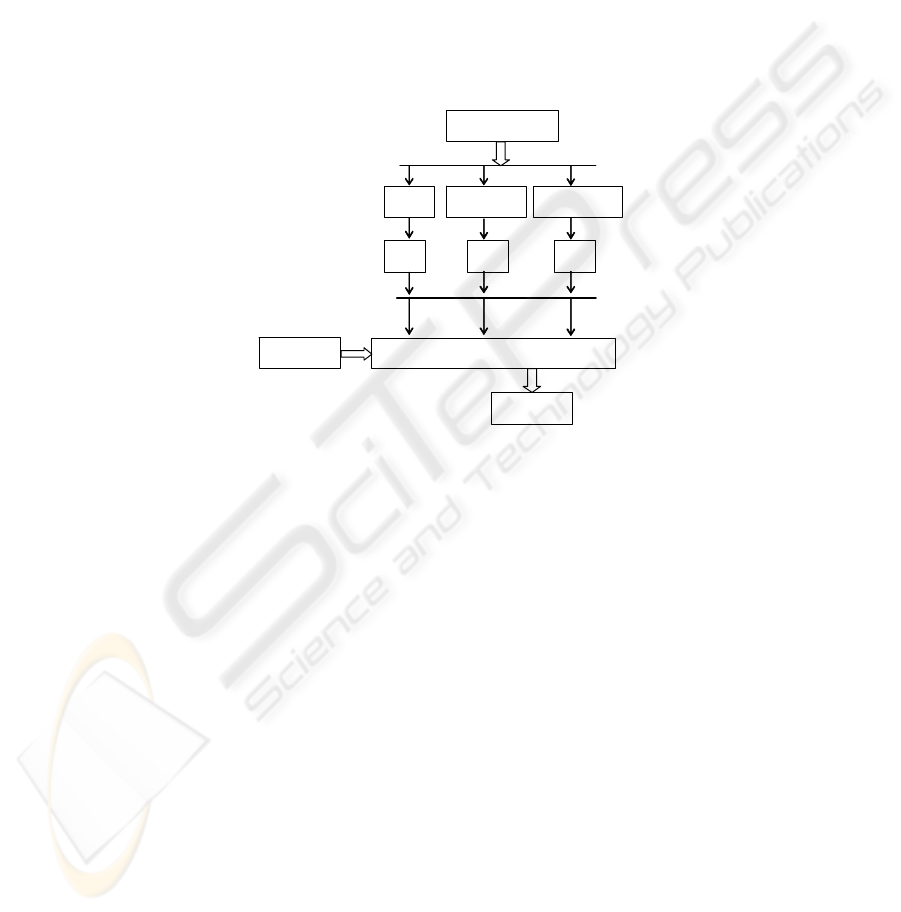
The proposed ensemble begins by creating a set of three experts (NB, WINNOW,

Voted Perceptron classifiers). When a new instance arrives, the algorithm passes it to

and receives a prediction from each expert. In online setting, the algorithm continu-

ally modifies its hypothesis as it is being used; it repeatedly receives a pattern, pre-

dicts its classification based on majority vote of the expert predictions, finds out the

correct classification, and possibly updates its hypothesis accordingly. The proposed

ensemble is schematically presented in Fig. 1, where hi is the produced hypothesis of

each classifier, x the instance for classification and y* the final prediction of the pro-

posed online ensemble. The number of model or runtime parameters to be tuned by

the user is an indicator of an algorithm’s ease of use. For a non specialist in data min-

ing, the proposed ensemble with no user-tuned parameters will certainly be more

appealing.

Application

phase

Treaining set

Vot. Perc.

WINNOW

(x, ?)

h* = SumRule(h

, h

)

(x, y*)

Learnin

phase

Fig. 1. The proposed ensemble

It must be mentioned that WINNOW and Voted Perceptron are binary algorithms,

thus we made the use of error-correcting output coding (ECOC), or in short output

coding approach to reduce a multi-class problem to a set of multiple binary classifica-

tion problems (Dietterich and Bakiri, 1995). Output coding for multi-class problems

is composed of two stages. In the training stage we construct multiple independent

binary classifiers each of which is based on a different partition of the set of the labels

into two disjoint sets. In the second stage, the classification part, the predictions of the

binary classifiers are combined to extend a prediction on the original label of a test

instance.

It must also be mentioned that the proposed ensemble can easily be parallelized us-

ing a learning algorithm per machine. Parallel and distributed computing is of most

importance for Machine Learning (ML) practitioners because taking advantage of a

parallel or a distributed execution a ML system may: i) increase its speed; ii) increase

the range of applications where it can be used (because it can process more data, for

example).

4 Comparisons and Results

For the purpose of our study, hand selected datasets from real world problems with

varying characteristics. The datasets come from many domains of the UCI repository

[4] and covers areas such as: pattern recognition (iris, mushroom, vote, zoo), image

recognition (ionosphere, sonar), medical diagnosis (breast-cancer, breast-w, colic,

diabetes, heart-c, heart-h, heart-statlog, hepatitis, haberman, lymphotherapy, sick)

commodity trading (credit-a, credit-g) and various applications (waveform). There is

a brief description of these datasets in [4]. The used datasets are batch datasets, i.e.,

there is no natural order in the data. The most common way to convert the online

ensemble into a batch algorithm is to repeatedly cycle through a dataset, processing

the examples one at a time until the end of the dataset.

In order to calculate the classifiers’ accuracy, the whole training set was divided

into ten mutually exclusive and equal-sized subsets and for each subset the classifier

was trained on the union of all of the other subsets. Then, cross validation was run 10

times for each algorithm and the median value of the 10-cross validations was calcu-

lated. The WINNOW and Voted Perceptron algorithms are able to process symbolic,

categorical data only. However, the used datasets involve both symbolic and numeri-

cal features. Therefore, there was the important issue to discretize numerical (con-

tinuous) features. Entropy discretization method was used [8]. Entropy discretization

recursively selects the cut-points minimizing entropy until a stopping criterion based

on the Minimum Description Length criterion ends the recursion.

During the first experiment, each online learning algorithm (Naïve Bayes, Voted

Perceptron, WINNOW) is compared with the proposed ensemble.

It must be mentioned that we used the free available source code for these algo-

rithms by [20] for our experiments. We have tried to minimize the effect of any ex-

pert bias by not attempting to tune any of the algorithms to the specific dataset.

Wherever possible, default values of learning parameters were used. This approach

may result in lower estimates of the true error rate, but it is a bias that affects all the

learning algorithms equally.

In the last rows of the Table 1 there are the aggregated results. In Table 1, we rep-

resent with “vv” that the proposed ensemble looses from the specific algorithm. That

is, the specific algorithm performed statistically better than the proposed according to

t-test with p<0.001. In addition, in Table 1, we represent with “v” that the proposed

algorithm looses from the specific algorithm according to t-test with p<0.05. Fur-

thermore, in Table 1, “**” indicates that proposed ensemble performed statistically

better than the specific classifier according to t-test with p<0.001 while “*” according

to p<0.05. In all the other cases, there is no significant statistical difference between

the results (Draws). It must be mentioned that the conclusions are mainly based on

the resulting differences for p<0.001 because a p-value of 0.05 is not strict enough, if

many classifiers are compared in numerous datasets [16]. However, as one can easily

observe the conclusions remain the same with p<0.05.

In the last rows of the Table 1 one can also see the aggregated results in the form

(a, b, c). In this notation “a” means that the proposed ensemble is significantly less

accurate than the compared algorithm in a out of 28 datasets, “c” means that the pro-

posed algorithm is significantly more accurate than the compared algorithm in c out

of 28 datasets, while in the remaining cases (b), there is no significant statistical dif-

ference between the results.

Table 1. Comparing the proposed ensemble with the based online classifiers

Voting online

ensemble

WINNOW Voted

Perceptron

audiology 72.64 40.24** 48.71** 72.64

badges 99.93 100 99.83 99.66

balance 85.34 61.65 ** 75.12 ** 90.53 vv

breast-cancer 72.48 61.96 * 71.67 72.7

breast-w 96.61 94.68 96.3 96.07

Colic 82.23 76.61 * 82.2 78.7

Credit-a 84.06 76.78 * 85.52 77.86 **

credit-g 75.07 64.55 * 74.41 75.16

Diabetes 75.56 68.62 * 75.5 75.75

Haberman 73.1 71.77 72.41 75.06

heart-c 83.73 69.38 ** 80.79 83.34

heart-h 84.5 65.38 ** 81.98 83.95

heart-statlog 83.41 77.22 * 81.85 83.59

Hepatitis 84.01 74.91 * 82.93 83.81

Ionosphere 91.08 87.82 * 89.8 82.17 **

Iris 95.33 80.6 * 94.27 95.53

Labor 90.07 79.03 * 86.13 93.57

Lymphotherapy 83.01 67.55 * 78.74 83.13

Monk3 92.63 79.57 * 88.19 93.45

primary-tumor 49.77 20.73 ** 13.52 ** 49.71

Sick 96.95 92.16 ** 97.56 92.75 **

sonar 73.93 67.78 74.22 67.71 *

Soybean 92.93 68.91 ** 78.76 ** 92.94

titanic 77.85 63.09 ** 77.93 77.85

vote 94.04 91.26 94.82 90.02 **

Waveform 82.36 65.81 ** 81.8 80.01 **

wine 97.63 89.63 * 95.61 97.46

Zoo 95.07 79.91 ** 87.02 * 94.97

Average error 84.48 72.77 80.27 83.57

W-D-L (p<0.001) 0/18/10 0/24/4 1/22/5

W-D-L (p<0.05) 0/5/23 0/23/5 1/21/6

To sum up, the proposed ensemble is significantly more precise than WINNOW

algorithm in 10 out of the 28 datasets, whilst it has significantly higher error rates in

none dataset. In addition, the proposed algorithm is significantly more accurate than

Voted Perceptron algorithms in 4 out of the 28 datasets, whereas it has significantly

higher error rates in none dataset. Moreover, the proposed ensemble is significantly

more precise than NB algorithm in 5 out of the 28 datasets, whilst it has significantly

higher error rates in one dataset.

During the second experiment, a representative algorithm for each of batch sophis-

ticated machine learning techniques was compared with the proposed ensemble. We

used batch algorithms as an upper measure of the accuracy of learning algorithms.

Most of the incremental versions of batch algorithms are not lossless [18], [15], [19].

A lossless online learning algorithm is an algorithm that returns a hypothesis identical

to what its corresponding batch algorithm would return given the same training set.

The C4.5 algorithm [14] was the representative of the decision trees in our study. The

most well-known learning algorithm to estimate the values of the weights of a neural

network - the Back Propagation (BP) algorithm [12] - was the representative of the

neural nets. In our study, we also used the 3-NN algorithm that combines robustness

to noise and less time for classification than using a larger k for kNN [1]. Finally, the

RIPPER [5] was the representative of the rule learners in our study.

Table 2. Comparing the proposed ensemble with well known classifier

Voting online

ensemble

C4.5 3NN RIPPER BP

audiology 72.64 77.26 67.97 72.57 43.82 **

badges 99.93 100 100 100 100

balance 85.34 77.82** 86.74 80.91* 85.67

breast-cancer 72.48 74.28 73.13 71.65 71,18

breast-w 96.61 95.01* 96.61 95.72 95,97

Colic 82.23 85.16 80.95 84.97 82,58

credit-a 84.06 85.57 84.96 85.33 85.94

credit-g 75.07 71.25* 72.21 71.86 72,75

Diabetes 75.56 74.49 73.86 75.22 74.64

Haberman 73.1 71.05 69.77 72.43 76,56

heart-c 83.73 76.94* 81.82 79.05 81,39

heart-h 84.5 80.22* 82.33 79.26 * 81,37

heart-statlog 83.41 78.15* 79.11 78.70 82,11

Hepatitis 84.01 79.22 80.85 77.43 * 81,3

Ionosphere 91.08 89.74 86.02* 89.30 85,84*

Iris 95.33 94.73 95.20 93.93 96,27

Labor 90.07 78.60 92.83 83.37 88,57

Lymphotherapy 83.01 75.84 81.74 77.36 80,24

Monk3 92.63 92.95 86.72 83.99* 88.69

primary-tumor 49.77 41.39** 44.98* 38.59 ** 28,11**

Sick 96.95 98.72 v 96.21 98.30 v 96,78

sonar 73.93 73.61 83.76 v 75.45 73.3

Soybean 92.93 91.78 91.2 91.93 33,43**

titanic 77.85 78.55 78.9 77.97 78.25

vote 94.04 96.57v 93.08 95.7 96.32

Waveform 82.36 75.25 ** 77.67** 79.14** 59.62**

wine 97.63 93.2 * 95.85 92.48* 83.08 **

Zoo 95.07 92.61 92.61 87.03 * 61,21**

Average error 84.48 82.14 83.11 81.77 77.32

W-D-L

(p<0.001)

0/25/3 0/27/1 0/26/2 0/22/6

W-D-L (p<0.05) 2/17/9 1/24/3 1/19/8 0/21/7

As one can see in Table 2, the proposed ensemble is significantly more precise

than BP algorithm with one hidden layer in 6 out of the 28 datasets, whilst it has

significantly higher error rates in none dataset. In addition, the proposed algorithm is

significantly more accurate than 3NN algorithms in 1 out of the 28 datasets, whereas

it has significantly higher error rates in none dataset. The proposed algorithm is also

significantly more precise than RIPPER algorithm in 2 out of the 28 datasets, while it

has significantly higher error rates in none dataset. Finally, the proposed algorithm

has significantly lower error rates than C4.5 algorithm in 3 out of the 28 datasets and

it is significantly less accurate in none dataset

All the experiments indicate that the proposed ensemble performed, on average,

better than all the tested algorithms using less time for training, too. Clearly, incre-

mental updating would be much faster than rerunning a batch algorithm on all the

data seen so far, and may even be the only possibility if all the data seen so far cannot

be stored or if we need to perform online prediction and updating in real time or, at

least, very quickly. We are much interested in minimizing the required training time

because, as we have already said, a major research area is the exploration of accurate

techniques that can be applied to problems with millions of training instances, thou-

sands of features, and hundreds of classes. It is desirable to have machine-learning

techniques that can analyze large datasets in just a few hours of computer time.

5 CONCLUSION

Online learning is the area of machine learning concerned with learning each training

example once (perhaps as it arrives) and never examining it again. Online learning is

necessary when data arrives continuously so that it may be impractical to store data

for batch learning or when the dataset is large enough that multiple passes through the

dataset would take too long.

Ideally, we would like to be able to identify or design the single best learning algo-

rithm to be used in all situations. However, both experimental results and theoretical

work indicate that this is not possible [12]. Recently, the concept of combining classi-

fiers is proposed as a new direction for the improvement of the classification accu-

racy. However, most ensemble algorithms operate in batch mode. There are several

avenues that could be explored when designing an online ensemble algorithm. A

naive approach is to maintain a dataset of all observed instances and to invoke an

offline algorithm to produce an ensemble from scratch when a new instance arrives.

This approach is often impractical both in terms of space and update time for online

settings with resource constraints. To help alleviate the space problem we could limit

the size of the dataset by only storing and utilizing the most recent or most important

instances. However, the resulting update time is still often impractical.

For this reason, we have proposed an online ensemble that combines three online

classifiers: the Naive Bayes, the Voted Perceptron and the Winnow algorithms using

the voting methodology. We performed a large-scale comparison with other state-of-

the-art algorithms and ensembles on 28 standard benchmark datasets and we took

better accuracy in most cases. However, in spite of these results, no general method

will work always.

We have mostly used our online ensemble algorithm to learn static datasets, i.e.,

those which do not have any temporal ordering among the training examples. Much

data mining research is concerned with finding methods applicable to the increasing

variety of types of data available—time series, spatial, multimedia, worldwide web

logs, etc. Using online learning algorithms on these different types of data is an im-

portant area of future work. Moreover, the used combination strategy is based on

voting method. In a future work, apart from voting, it might be worth to try other

combination rules to find the regularity between the combination strategy, individual

classifiers and the datasets.

References

1. Aha, D., Lazy Learning. Dordrecht: Kluwer Academic Publishers (1997).

2. Auer P. & Warmuth M., Tracking the Best Disjunction, Machine Learning 32 (1998) 127–

150, Kluwer Academic Publishers.

3. Bauer, E. & Kohavi, R., An empirical comparison of voting classification algorithms:

Bagging, boosting, and variants. Machine Learning 36 (1999) 105–139.

4. Blake, C.L. & Merz, C.J, UCI Repository of machine learning databases. Irvine, CA:

University of California, Department of Information and Computer Science (1998):

[http://www.ics.uci.edu/~mlearn/MLRepository.html]

5. Cohen W., Fast Effective Rule Induction. In Proc. of Int Conf. of ML-95 (1995). 115-123.

6. Domingos P. & Pazzani M., On the optimality of the simple Bayesian classifier under

zero-one loss. Machine Learning, 29 (1997) 103-130.

7. Fan W., Stolfo S., and Zhang J., The application of AdaBoost for distributed, scalable and

on-line learning, in Proceedings of the Fifth ACM SIGKDD International Conference on

Knowledge Discovery and Data Mining. New York, NY: ACM Press, 1999, pp. 362-366.

8. Fayyad U., and Irani K., Multi-interval discretization of continuous-valued attributes for

classification learning. In Proc. of the 13

Int. Joint Conference on AI (1993) 1022-1027.

9. Fern, A., & Givan, R., Online ensemble learning: An empirical study. In Proceedings of

the Seventeenth International Conference on ML (2000) 279–286. Morgan Kaufmann.

10. Freund Y., Schapire R., Large Margin Classification Using the Perceptron Algorithm,

Machine Learning 37 (1999) 277–296, Kluwer Academic Publishers.

11. Littlestone N. & Warmuth M., The weighted majority algorithm. Information and Compu-

tation 108 (1994) 212–261.

12. Mitchell, T., Machine Learning. McGraw Hill (1997).

13. Oza, N. C. and Russell, S., Online Bagging and Boosting." In Artificial Intelligence and

Statistics 2001, eds. T. Richardson and T. Jaakkola, 105-112.

14. Quinlan J.R., C4.5: Programs for machine learning. Morgan Kaufmann, San Francisco

(1993).

15. Saad, D., Online learning in neural networks, London, Cambridge University Press

(1998).

16. Salzberg, S., On Comparing Classifiers: Pitfalls to Avoid and a Recommended Approach,

Data Mining and Knowledge Discovery 1 (1997) 317–328.

17. Schaffer, C., Selecting a classification method by cross-validation. Machine Learning 13

(1993) 135-143.

18. Utgoff, P., Berkman, N., & Clouse, J., Decision tree induction based on efficient tree

restructuring. Machine Learning, 29 (1997) 5–44.

19. Widmer G. and Kubat M., Learning in the presence of concept drift and hidden contexts.

Machine Learning 23 (1996) 69–101.

20. Witten I. & Frank E., Data Mining: Practical Machine Learning Tools and Techniques

with Java Implementations, Morgan Kaufmann, San Mateo (2000).