
AHP-Based
Classifier Combination
L
´
aszl
´
o Felf
¨
oldi and Andr
´
as Kocsor
1
Department of Informatics, University of Szeged, H-6720 Szeged,
´
Arp
´
ad t
´
er 2., Hungary
2
Research Group on Artificial Intelligence of the Hungarian Academy of Sciences and
University of Szeged, H-6720 Szeged, Aradi v
´
ertan
´
uk tere 1., Hungary
Abstract. Classifier combinations are effective techniques for difficult pattern
recognition problems such as speech recognition where the combination of dif-
ferently trained classifiers can produce a more robust phoneme classification on
noisy datasets. In this paper we investigate traditional linear combination schemes
(e.g. arithmetic mean and least squares methods), and propose a new combiner
based on the Analytic Hierarchy Process (AHP), a method frequently applied
in mathematical psychology and multi-criteria decision making. In addition, we
experimentally compare the applicability of these linear combination schemes
using neural network classifiers on a speech recognition framework and two test
sets from the UCI repository.
1 Introduction
In pattern recognition problems [1][2][3] the main aim is to construct a classifier (or
inducer) in order to model the behavior of a system. For each pattern of a pattern space
the classifier has to select a class label from the set of available labels. The construction
of a classifier (i.e. the learning process) is based on a set of labelled examples, and
strongly depends on prior knowledge about the pattern space and the characteristics
of the given examples. Given infinite training data, consistent classifiers approximate
the Bayesian decision boundaries to arbitrary precision, therefore providing a similar
generalization. However, often only a limited portion of the pattern space is available
or observable. Given a finite and noisy data set, different classifiers typically provide
different generalizations. It is thus necessary to train more networks when dealing with
classification problems to ensure that a good model or parameter set is found. However,
selecting such a classifier is not necessarily the ideal choice since potentially valuable
information may be wasted by discarding the results of the other classifiers. In order
to avoid this kind of loss of information, the output of all available classifiers should
be examined for the final decision. This approach is particularly useful for difficult
problems such as those that involve a large amount of noise.
A fair number of combination methods have been proposed in the literature [4]
which have proved effective in improving classifier performance. In this paper we focus
on linear combination schemes, especially averaging techniques. Experimental studies
have shown that linear classifier combinations can improve the recognition accuracy.
Felföld L. and Kocsor A. (2004).
AHP-Based Classifier Combination.
In Proceedings of the 4th International Workshop on Pattern Recognition in Information Systems, pages 45-58
DOI: 10.5220/0002680200450058
Copyright
c
SciTePress
Tumer and Ghosh showed that combining networks using single averaging reduces the
variance of the actual decision boundaries around the optimum boundary [5]. Later
Fumera and Roli extended the theoretical framework for the weighted averaging rule
[6]. However, these theoretical explanations apply very restrictive assumptions, hence
they cannot show the real performance of the combiner. To improve the accuracy of the
averaging techniques, we propose a new combination method based on the Analytical
Hierarchy Process, and demontrate that it may produce a more robust classification
performance in tests
The paper is organized as follows. In the next section we give a brief overview of
linear combination schemes, including averaging techniques, and examine the theoret-
ical background of these systems. The third section introduces the Analytic Hierarchy
Process and shows utilization facilities provided in combination frameworks. The ex-
perimental section then compares the performance of various linear schemes on differ-
ent database and classifier sets. Finally, we give some brief conclusions and ideas for
future research.
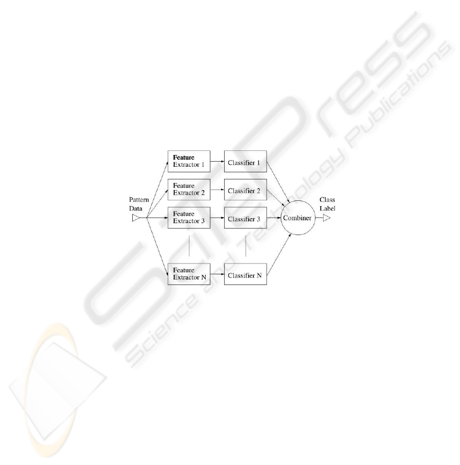
2 Linear Classifier Combinations
Fig.1. General parallel combination scheme
Combiners aggregate the outputs of different classifiers to make a final decision.
This aggregation depends on the kind of information that the individual classifiers can
supply. From this viewpoint the classification methods can be grouped into three main
categories:
1. Measurement or Confidence. The classifier can model probability values for each
class label. Let f
j
i
(x) denote the output of classifier C
j
for class i and pattern x.
The linear combination method can be described by the formula
ˆ
f
i
(x) =
N
X
j=1
w
j
f
j
i
(x), (1)
46

where
ˆ
f
i
(x) is the combined class conditional probability, and w
j
is the weighting
factor of classifier C
j
. The final decision can be obtained by selecting the class with
the greatest probability, in accordance with the Bayesian decision principle.
2. Ranking. The classifier can produce a list of class labels in the order of their prob-
abilities. The combined position ˆg
i
is then computed via the formula
ˆg
i
(x) =
N
X
j=1
w
j
g
j
i
(x), (2)
where g
j
i
(x) is the position of the label i in the classification result of pattern x
obtained by the classifier C
j
. With the selection of a proper monotonic decreasing
function u, and
f
j
i
(x) = u(g
j
i
(x)), (3)
the ranking-type combination can be reduced to the confidence-type scheme.
3. Abstract. The classifier supplies only the most probable class label. In this case the
combination relies on the majority voting formula
ˆ
L(x) = arg max
i
X
L
j
(x)=i
w
j
, (4)
where L
j
(x) is the index of the class label calculated for pattern x. Taking the
selection of f
j
i
(x) as
f
j
i
(x) =
½
1 L
j
(x) = i
0 otherwise
(5)
leads to the reformulation of voting as a confidence-type combination much like
that for the ranking type.
As we have shown, the output of classifiers belonging to the Ranking or Abstract class
can be transformed to class conditional probability values. Therefore, in the follow-
ing section we shall deal only with the confidence-type combination, and expect the
combiners to supply the class conditional probabilities.
We commence our study of linear combinations with a theoretical investigation, and
then show how to apply them in practice.
2.1 Theoretical investigation
As mentioned previously, the output of the classifiers are expected to approximate the
corresponding a posteriori probabilities if they are reasonably well trained. Thus the
decision boundaries obtained using this kind of classifier are close to Bayesian decision
boundaries. Tumer and Ghosh developed a theoretical framework for analyzing the av-
eraging rule of linear combinations [5]. Later Roli and Fumera extended this concept
by examining the weighted averaging rule [6].
We shall focus on the classification performance near these decision boundaries.
Consider the boundary between class i
1
and i
2
. The output of the classifier is
47

f
i
(x) = p
i
(x) + ²
i
(x) (6)
where p
i
(x) is the real a posteriori probability of class i, and ²
i
(x) is the estimation
error. Let us assume that the class boundary x
b
obtained from the approximated a pos-
teriori probabilities
f
i
1
(x
b
) = f
i
2
(x
b
) (7)
are close to the Bayesian boundaries x
∗
, i.e.
p
i
1
(x
∗
) = p
i
2
(x
∗
), (8)
for boundary between class i
1
and i
2
. Additionally assuming that the estimated errors
²
i
(x) on different classes are independently and identically distributed (i.i.d.) variables
with zero mean, Tumer and Ghosh showed that the expected error of classification can
be expressed as:
E = E
Bayes
+ E
add
, (9)
where E
Bayes
is the error of a classifier with the correct Bayesian boundary. The added
error E
add
can be expressed as:
E
add
=
sσ
2
b
2
, (10)
where σ
2
b
is the variance of b,
b =
²
i
1
(x
b
) − ²
i
2
(x
b
)
s
, (11)
and s is a constant term depending on the derivatives of the probability density functions
at the optimal decision boundary.
Let us consider the effect of combining multiple classifiers. We shall deal only with
linear combinations, so we have the following combined probabilities:
ˆ
f
i
(x) =
N
X
j=1
w
j
f
j
i
(x), (12)
where f
j
i
denotes the output of the classifier C
j
for the class i. Assuming normalized
weights, i.e.
N
X
j=1
w
j
= 1, w
j
≥ 0 (13)
we have that
ˆ
f
i
(x) = p
i
(x) + ˆ²
i
(x), (14)
48

where
ˆ²
i
(x) =
N
X
j=1
w
j
²
j
i
(x) (15)
Let us compute the variance of
ˆ
b, where
ˆ
b =
ˆ²
i
1
− ˆ²
i
2
s
. (16)
Assuming that ²
j
i
(x) are i.i.d. variables with zero mean and variance σ
2
²
j
, the errors of
different classifiers on the same class are correlated, while on different classes they are
uncorrelated.
Cov(²
m
i
1
(x
b
), ²
n
i
2
(x
b
)) =
½
ρ
mn
when i
1
= i
2
0 otherwise
,
where ρ
mn
denotes the covariance between the errors of classifier C
m
and C
n
for each
class. Expanding the tag σ
2
²
in Eq. (10), we find that
ˆ
E
add
=
1
s
N
X
j=1
w
2
j
σ
2
²
j
+
1
s
X
m6=n
w
m
w
n
ρ
mn
.
Expressed in terms of additional errors of the classifiers
ˆ
E
add
=
1
s
N
X
j=1
w
2
j
E
j
add
+
1
s
X
m6=n
w
m
w
n
ρ
mn
,
where the term E
j
add
denotes the added error of the classifier C
j
. In the case of uncor-
related estimation errors (i.e. when ρ
mn
= 0), this equation reduces to
ˆ
E
add
=
N
X
j=1
w
2
j
E
j
add
, (17)
which leads to the following optimal values for w:
w
j
= c
1
E
j
add
, (18)
where c is a normalization factor. With equally performing classifiers, that is when all
the errors E
j
add
have the same value
E
j
add
= E
add
, j = 1, . . . , N, (19)
49

we obtain the Simple Averaging rule:
w
j
=
1
N
, (20)
which results in the following error value:
ˆ
E
add
=
1
N
E
add
. (21)
This formula shows that, under the conditions mentioned, linear combinations reduce
the error of the individual classifier. Considering correlated errors, however, does not
lead to a simple general expression for optimal values of weights, and other methods
are required to estimate the optimal parameters.
2.2 Construction
To achieve the best combination performance the parameters of the combiner can be
trained on a selected training data set. The form of linear combinations we deal with is
quite simple (see Figure 1), the trainable parameters being just the weights of classifiers.
Thus the various linear combinations differ only in the values of these factors. In the
following we give some examples of methods commonly employed, and in the next
section we propose a new method for computing these parameters.
1. Simple Averaging. In this simplest case, the weights can be selected so they have
the same value:
w
j
=
1
N
. (22)
As mentioned before, this selection is optimal when all the classifiers have a very
similar performance, and all the assumptions mentioned in Section 2.1 hold.
2. Weighted Averaging. Experiments show [6] that Simple Averaging can be out-performed
when selecting weights to be inversely proportional to the error rate of the corre-
sponding classifier:
w
j
=
1
E
j
, (23)
where E
j
is the error rate of the classifier C
j
, i.e. the ratio of the number of correctly
classified patterns and total number of patterns on a selected data set for training
the combiner. This rule (a more general version of the Simple Averaging rule) is
employed in order to handle the combination of unequally performing classifiers.
3. Least-squares methods. To calculate the weights w
j
one can take those values that
minimize the distance between the computed and estimated class conditional prob-
abilities:
min
w
X
x∈X
l
X
i=1
N
X
j=1
w
j
f
j
i
(x) − p
i
(x)
2
, (24)
where
X = {x
1
, . . . , x
m
}
50
is the training set of patterns for the combination, and p
i
(x) is the estimated class
conditional probability function. In the case of supervised learning the class labels
are available for all the training patterns, but there is no direct way of comparing
this information with computed a posteriori probabilities. Assuming a Bayesian
decision, the pattern x has the label L(x) = i when p
i
(x) ≥ p
j
(x) for all i 6= j.
Let us approximate p
i
(x) by
p
i
(x) =
½
1 if L(x) = i
0 otherwise
, (25)
or calculate it from the error correlation matrix of the n combiners [7]. Using matrix
notations the problem described in Eq. (24) can be expressed as:
min
w
(Aw − b)
T
(Aw − b), (26)
where
a
j,(mi+k)
= f
j
i
(x
k
),
b
mi+k
= p
i
(x
k
),
This optimization problem leads to the following linear equation:
A
T
A w = A
T
b, (27)
which provides a way of determining the weighting factors.
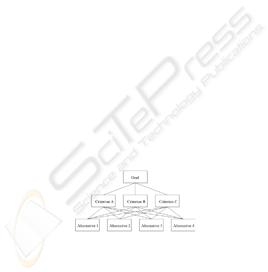
3 The Analytic Hierarchy Process
Analytic Hierarchy Process is an intuitive and efficient method for multi-criteria decision-
making (MCDM) applications [8]. The structure of a typical decision problem (see Fig.
2) consists of alternatives and decision criteria. Each alternative can be evaluated in
terms of the decision criteria and, in the case of multilevel criteria, the relative impor-
tance (or weight) of each criterion can also be estimated.
Fig.2. A simple application of AHP
In the following we give a brief summary of the fundamental properties of the AHP,
and propose a combination method based on it.
51

3.1 Mathematical model
The first step of AHP is to divide the decision problem into sub-problems, which are
structured into hierarchy levels. The number of levels depends on the complexity of the
initial problem. The leaves contain the possible alternatives and the inner nodes repre-
sent the criteria. To compute the importance of possible choices, pairwise comparison
matrices are utilized for each criterion. The element a
ij
of the comparison matrix A
represents the relative importance of choice i against the choice j, implying that the
element a
ji
is the reciprocal of a
ij
. Let the importance value v of choice y be expressed
as a linear combination of the importance values for each applied criterion:
v(y) =
n
X
j=1
w
j
v(y
j
), (28)
where w
j
is the importance of choice y with respect to the criterion y
j
. Using compar-
ison matrices AHP propagates the importance values of each node from the topmost
criteria towards the alternatives, and selects the alternative with the greatest importance
value as its final decision.
Let us now focus on the computation of the weights w for a selected criterion. The
elements of a given pairwise comparison matrix approximate the relative importance of
the choices, thus
a
ij
≈
w
i
w
j
, (29)
where the elements of the unknown vector w are the importance values. A matrix M is
called consistent if its components satisfy the following equalities:
m
ij
=
1
m
ji
, (30)
and
m
ij
= m
ik
m
kj
∀ i, j, k. (31)
If A is not consistent, it is not possible to find a vector w that satisfies the equation
a
ij
=
w
i
w
j
. (32)
Now let us define the matrix of weight ratios by
W =
w
1
w
1
w
1
w
2
w
1
w
3
· · ·
w
1
w
n
w
2
w
1
w
2
w
2
w
2
w
3
· · ·
w
2
w
n
w
3
w
1
w
3
w
2
w
3
w
3
· · ·
w
3
w
n
.
.
.
.
.
.
.
.
.
.
.
.
.
.
.
w
n
w
1
w
n
w
2
w
n
w
3
· · ·
w
n
w
n
, (33)
or, in matrix notation,
W = ww
T
. (34)
52

Note that Eqs. (30) and (31) hold for the matrix W :
w
ij
=
w
i
w
j
=
w
i
w
k
w
k
w
j
= w
ik
w
kj
, (35)
hence the matrix of weight ratios is consistent.
Because the rows of matrix W are linearly dependent, the rank of the matrix is 1,
and there is only one nonzero eigenvalue. Knowing that the trace of a matrix is invariant
under similarity transformations, the sum of diagonal elements is equal to the sum of
eigenvalues, which implies that the nonzero eigenvalue λ
max
equals the number of the
rows:
λ
max
= n. (36)
It is straightforward to check that the vector w is an eigenvector of matrix W corre-
sponding to the maximum eigenvalue
(W w)
i
=
n
X
j=1
W
ij
w
j
=
n
X
i=1
w
i
w
j
w
j
=
n
X
j=1
w
i
= nw
i
.
The aim of AHP is to resolve the weight vector w from a pairwise comparison
matrix A, where the elements of A corresponds to the measured or estimated weight
ratios. Following Saaty we shall assume that
a
ij
> 0, (37)
and
a
ij
=
1
a
ji
. (38)
From matrix theory it is known that a small perturbation of the coefficients implies a
small perturbation of the eigenvalues. Hence we still expect to find an eigenvalue close
to n, and select the elements of the corresponding eigenvector as weights. It can be
proved that
λ
max
≥ n,
and the matrix A is consistent if and only if λ
max
= n. A way of measuring the
consistency of the matrix A is by defining the consistency index (CI) as the negative
average of the remaining eigenvalues:
CI =
X
λ<λ
max
λ
n − 1
=
λ
max
− n
n − 1
(39)
53

3.2 Combination using AHP
As mentioned above, AHP provides the following solution for the problem of linear
MCDM systems:
v(y) =
n
X
i=1
w
i
v(y
i
),
where the importance value of the choice is the linear combination of the importance
values of the direct criteria. In linear classifier combinations the combined class condi-
tional probabilities are computed as weighted sums of the probability values from each
classifier, so
f
i
(x) =
N
X
j=1
w
j
f
j
i
(x).
Noting the similarities between these two methods, it is clear that, by applying pair-
wise comparisons on classifiers performance, AHP provides a way of computing the
weights of inducers in classifier combinations. Let us calculate the element a
ij
of the
comparison matrix as the quotient of classification performance on a selected test data
set:
a
ij
=
1
E
i
1
E
j
=
1
a
ji
, (40)
where E
i
is the classification error of classifier C
i
. If all the performance errors are
measured on the same test data set, the comparison matrix A is consistent, and the
elements of the eigenvector whose corresponding eigenvalue is N, that is
w
i
=
1
E
i
, (41)
are the same those as generated by weighted averaging. However, this method allows us
to make pairwise comparisons of different inducers applied on different (e.g. randomly
generated) test sets, taking advantage of the stabilizing effect of AHP. This leads to
more a robust classification performance, especially in noisy environments, as shown
in the experimental section.
4 Experiments
In this section we describe our experiments for comparing the performance of averaging
combiners and our AHP-based combiner.
4.1 Evaluation Domain
In the experiments three data sets were employed: a data-set used in our speech recog-
nition system, and two other datasets (letter and satimage) originating from the stat-
log/UCI repository. (http://www.liacc.up.pt/ML/statlog)
54

1. Speech data set [9]. The database is based on recorded samples taken from 160
children aged between 6 and 8. The ratio of girls and boys was 50% - 50%.The
speech signals were recorded and stored at a sampling rate of 22050 Hz in 16-bit
quality. Each speaker uttered all the Hungarian vowels, one after the other, sepa-
rated by a short pause. Since we decided not to discriminate their long and short
versions, we only worked with 9 vowels altogether. The recordings were divided
into a train and a test set in a ratio of 50% - 50%. There are numerous methods for
obtaining representative feature vectors from speech data, but their common prop-
erty is that they are all extracted from 20-30 ms chunks or frames of the signal in
5-10 ms time steps. The simplest possible feature set consists of the so-called bark-
scaled filterbank log-energies (FBLE). This means that the signal is decomposed
with a special filterbank and the energies in these filters are used to parameterize
speech on a frame-by-frame basis. In our tests the filters were approximated via
Fourier analysis with a triangular weighting. Altogether 24 filters were necessary
to cover the frequency range from 0 to 11025 Hz. Although the resulting log-energy
values are usually sent through a cosine transformation to obtain the well-known
mel-frequency cepstral coefficients (MFCC), we abandoned it because, as we ob-
served earlier, the learner we work with is not sensitive to feature correlations so a
cosine transformation would bring no significant improvement.
2. Letter Data Set. The objective of the Data set is to identify each of a large number
of black-and-white rectangular pixel displays as one of the 26 capital letters in
the English alphabet. The character images were based on 20 different fonts and
each letter within these 20 fonts was randomly distorted to produce a file of 20,000
unique stimuli. Each stimulus was converted into 16 primitive numerical attributes
(statistical moments and edge counts) which were then scaled to fit into a range of
integer values from 0 to 15. We typically trained on the first 16000 items and then
used the resulting model to predict the letter category for the remaining 4000.
3. Satimage Data Set. One frame of Landsat MSS imagery consists of four digital
images of the same scene in different spectral bands. Two of these are in the visible
region (corresponding approximately to green and red regions of the visible spec-
trum) and two are in the (near) infra-red. Each pixel is a 8-bit binary word, with 0
corresponding to black and 255 to white. The spatial resolution of a pixel is about
80m x 80m. Each image contains 2340 x 3380 such pixels. The database is a (tiny)
sub-area of a scene, consisting of 82 x 100 pixels. Each line of data corresponds
to a 3x3 square neighborhood of pixels completely contained within the 82x100
sub-area. Each line contains the pixel values in the four spectral bands (converted
to ASCII) of each of the 9 pixels in the 3x3 neighborhood and a number indicating
the classification label of the central pixel. The number of possible class labels for
each pixel is 7. We trained on the first 4435 patterns of the database and selected
the remaining 2000 patterns for testing.
4.2 Evaluation Method
During the experiments we compared the performance of 6 different combiners applied
on each of the 3 databases. For each of the databases we trained 3-layered neural net-
55
works with different structures, and selected 5 subsets of classifiers, denoted by Set1
to Set5.
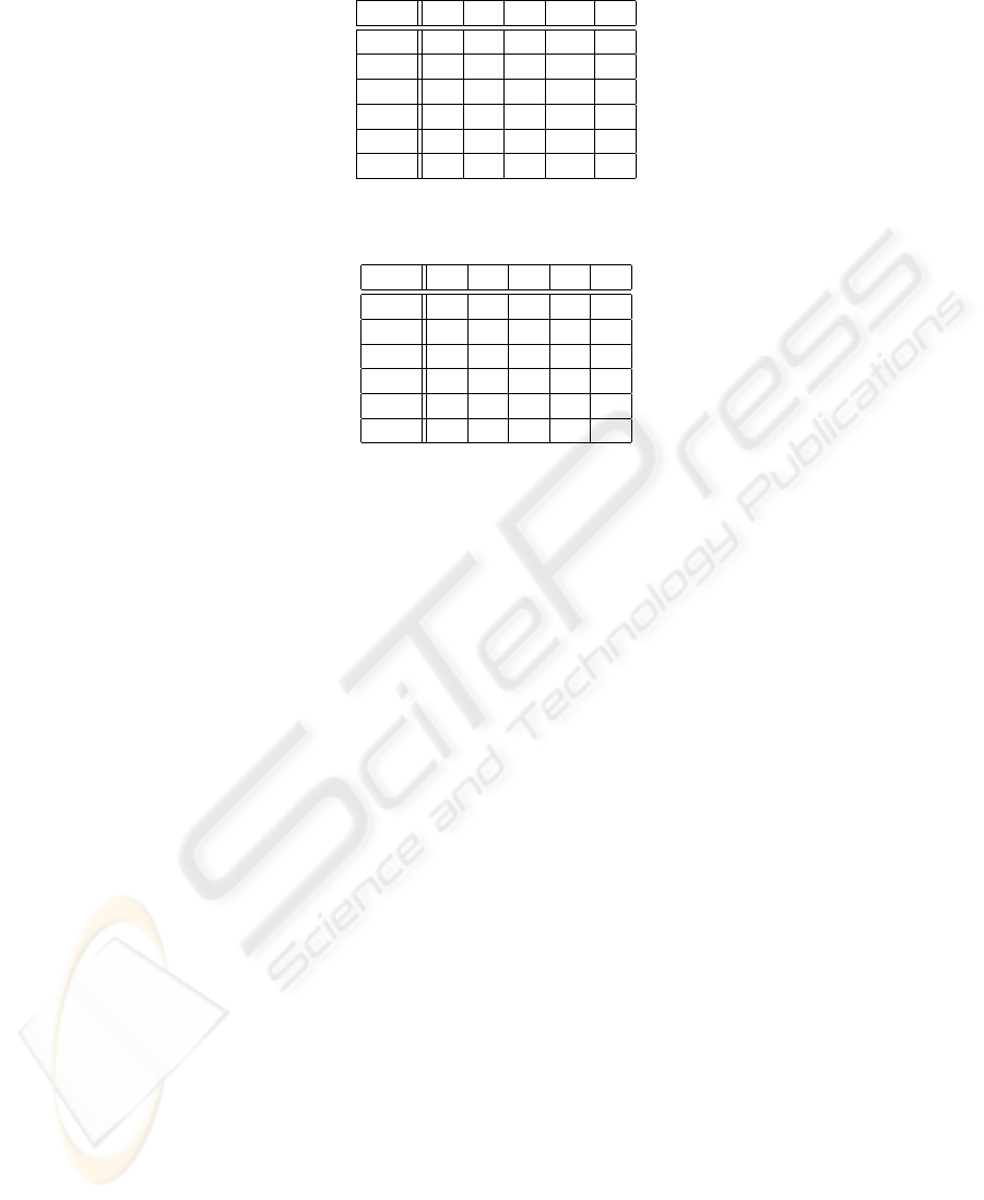
In the case of the speech and letter databases we trained networks setting the number
of neurons in the hidden layer to 5, 10, 20, 40, 80, 160, and 320. Table 1 shows the
construction of classifier sets. The columns refer to the number of hidden neurons, and
the rows show which networks belong to the selected classifier sets.
5 10 20 40 80 160 320
Set1 x x x x x x x
Set2 x x x x x x
Set3 x x x x x
Set4 x x x x
Set5 x x x
Table 1. Classifier sets for the speech and letter databases.
The satimage database contains only 7 classes. In this case we trained networks with
hidden layer size selected to 2, 5, 10, 20, 40, 80, and 160. The corresponding classifier
selection is displayed in Table 2.
2 5 10 20 40 80 160
Set1 x x x x x x x
Set2 x x x x x x
Set3 x x x x x
Set4 x x x x
Set5 x x x
Table 2. Classifier sets for the satimage database.
The experiments compared the performance of linear combination schemes with
different methods for acquiring the proper weights. We examined 2 schemes of Aver-
aging : SA and W A (i.e. simple and weighted) averaging, and 4 schemes of AHP.
To calculate the pairwise comparison matrices needed for the AHP method, we took
the quotient of classification errors of the two competing networks on a random test
set generated by bootstrapping (resampling the training data set with replacement) of
the training set. In accordance with the size of the generated test set we had 4 AHP
schemes, AHP 1 to AHP 4, setting the size of each to 50, 100, 200 and 400, respec-
tively. With the W A combiner, the original training set was selected for the calculation
of the weights.
56
Set1 Set2 Set3 Set4 Set5
SA 8.52 9.26 9.95 9.77 8.80
W A 8.66 9.21 9.91 9.81 8.75
AHP
1
8.66 8.94 9.44 10.05 8.80
AHP
2
8.56 9.12 9.72 10.19 8.80
AHP
3
8.61 9.21 9.49 9.58 8.70
AHP
4
8.61 9.31 9.55 9.07 8.70
Table 3. Classification errors [%] on the Speech database (Error without combination: 12.92%)
Set1 Set2 Set3 Set4 Set5
SA 8.70 8.34 7.88 7.26 7.78
W A 7.56 7.64 7.64 7.06 7.68
AHP
1
6.84 7.26 7.04 6.76 7.48
AHP
2
6.74 6.90 6.98 6.82 7.56
AHP
3
6.67 6.94 6.96 6.80 7.58
AHP
4
6.78 7.00 6.88 6.82 7.54
Table 4. Classification errors [%] on the Letter database (Error without combination: 13.78%)
4.3 Results and Discussion
Tables 3, 4, and 5 show the results of the experiments. Columns represent the various
classifier sets, while rows show the classification errors measured using the selected
combination of the corresponding classifier group.
As expected, all the combinations here improved the generalization performance of
the simple classifier. In almost every case AHP-based combinations outperformed the
weighed averaging combinations. However, in some cases SA performed better than
W A and the AHP combiners, showing that the strong assumptions of the method are
not always satisfied [10].
The performance of AHP combiners depends on the size of testing set. When the
test sets selected were too small, the measured accuracy values did not characterize the
goodness of the classifiers, and yielded wrong combination results. Increasing the size,
however, makes the consistency index (CI) tend to zero, producing weights that tend
to the values calculated by weighted averaging. Determining the optimal size of the test
set requires further study.
When considering the sensitivity for the selection of different classifier subsets,
the AHP-based combiner has a behavior similar to that of the W A method, hence the
optimal classifier set can be selected by methods available for the averaging combiners
[6].
Lastly, we should say that the AHP-based combination scheme is a good tool for
making the solution of the classification problem more accurate and reliable.
57

Set1 Set2 Set3 Set4 Set5
SA 10.95 10.35 10.35 10.00 10.05
W A 10.50 10.35 10.45 9.90 10.00
AHP
1
10.05 9.95 10.05 9.60 9.30
AHP
2
10.00 9.70 9.45 9.50 9.50
AHP
3
9.80 9.50 9.50 9.20 9.45
AHP
4
9.90 9.55 9.75 9.30 9.50
Table 5. Classification errors [%] on the Satimage database. (Error without combination: 12.05%)
5 Conclusion
In this paper we proposed a new linear combination method, and compared its per-
formance with those of other combiners. As shown in the experiments, AHP-based
combinations proved an effective generalization of the weighted averaging rule; they
outperformed the other averaging methods in almost every case.
Finally, we should mention that resampling techniques may further improve the
performance of linear combinations, hence it is worth investigating generalizations of
the bootstrapped learners Bagging [11] and Boosting [12] in future work.
References
1. Anil K. Jain, Robert P. W. Duin, and Jianchang Mao. Statistical pattern recognition: A review.
IEEE Transactions on Pattern Analysis and Machine Intelligence, 22(1):4–37, 2000.
2. V. N. Vapnik. Statistical Learning Theory. John Wiley and Son, 1998.
3. R. O. Duda, P. E. Hart, and D. G. Stork. Pattern Classification. John Wiley and Son, New
York, 2001.
4. L. Xu, A. Krzyzak, and C.Y. Suen. Method of combining multiple classifiers and their
application to handwritten numeral recognition. IEEE Trans. on SMC, 22(3):418–435, 1992.
5. K. Tumer and J. Ghosh. Analysis of decision boundaries in linearly combined neural classi-
fiers. Pattern Recognition, 29:341–348, 1996.
6. F. Roli and G. Fumera. Analysis of linear and order statistics combiners for fusion of imbal-
anced classifiers. In 3rd Int. Workshop on Multiple Classifier Systems (MCS 2002), Cagliari,
Italy, June 2002. Springer-Verlag, LNCS.
7. M. P. Perrone and L. N. Cooper. When networks disagree: Ensemble methods for hybrid neu-
ral networks. In R. J. Mammone, editor, Neural Networks for Speech and Image Processing,
pages 126–142. Chapman-Hall, 1993.
8. T. L. Saaty. The Analytic Hierarchy Process. McGraw-Hill, New York, 1980.
9. A. Kocsor and L. T
´
oth. Kernel-based feature extraction with a speech technology application.
In IEEE TRANS. ON SIGNAL PROCOCESSING, 2003.
10. G. Fumera and F. Roli. Linear combiners for classifier fusion: Some theoretical and experi-
mental results. In 4th Int. Workshop on Multiple Classifier Systems (MCS 2003), Guildford,
UK, January 2003. Springer-Verlag, LNCS.
11. Leo Breiman. Bagging predictors. Machine Learning, 24(2):123–140, 1996.
12. Freund. Boosting a weak learning algorithm by majority. In Proceedings of the Workshop
on Computational Learning Theory (COLT 1990). Morgan Kaufmann Publishers, 1990.
58
