
Comparison
of
Combination Methods using
Spectral Clustering Ensembles
Andr´e Louren¸co and Ana Fred
1
Instituto de Telecomunica¸c˜oes, IST , Portugal,
2
Instituto
de Telecomunica¸c˜oes, IST , Portugal,
Abstract. We address the problem of the combination of multiple data
partitions, that we call a clustering ensemble. We use a recent clustering
approach, known as Spectral Clustering, and the classical K-Means algo-
rithm to produce the partitions that constitute the clustering ensembles.
A comparative evaluation of several combination methods is performed
by measuring the consistency between the combined data partition and
(a) ground truth information, and (b) the clustering ensemble. Two con-
sistency measures are used: (i) an index based on cluster matching be-
tween two partitions; and (ii) an information theoretic index exploring
the concept of mutual information between data partitions. Results on
a variety of synthetic and real data sets show that, while combination
results are more robust solutions than individual clusterings, no combi-
nation method proves to be a clear winner. Furthermore, without the
use of a priori information, the mutual information based measure is
not able to systematically select the best combination method for each
problem, optimality being measured based on ground truth information.
1 INTRODUCTION
Let X = {x
1
, x
2
, . . . , x
n
} be a set of n objects, and S = {s
1
, . . . , s
n
} be a set of
vectors representing the data in a d-dimensional space, s
i
∈ R
d
. Many clustering
algorithms exist, producing distinct partitionings of the data. Let’s define clus-
tering ensemble as a set of N partitions, P = {P
1
, P
2
, . . . , P
i
, . . . , P
N
}, where
each partition, P
i
=
©
C
i
1
, C
i
2
, . . . , C
i
k
i
ª
, has k
i
clusters.
Inspired in the work of sensor fusion and classifier combination [1, 2], the idea
of combining data partitions produced by multiple algorithms or data represen-
tations has recently been proposed [3–5], trying to benefit from the strengths
of each algorithm, with the objective of producing a better solution than the
individual clusterings.
This framework, known as Combination of Clustering Ensembles, has many
strong points when compared to individual clustering algorithms, namely: ro-
bustness, overcoming instabilities of the individual clustering algorithms and/or
avoiding parameter selection; parallelization or distributed partition computa-
tion, improving scalability and the ability to deal with distributed clustering. To
Lourenço A. and Fred A. (2004).
Comparison of Combination Methods using Spectral Clustering Ensembles.
In Proceedings of the 4th International Workshop on Pattern Recognition in Information Systems, pages 222-233
DOI: 10.5220/0002688102220233
Copyright
c
SciTePress

apply this technique, relevant and challenging questions have to be addressed:
How to produce the partitions of the clustering ensemble? How to combine mul-
tiple partitions? How to validate the results?
The clustering ensemble can be produced in many different ways, including:
different algorithms [4]; different parameter values/initializations of a single al-
gorithm [6]; clustering different views/features of the data or manipulating the
data set, using techniques such as bootstrapping or boosting [7]. In this paper
we investigate the effect of combining clusterings produced by a single algo-
rithm with different initialization and/or parameter values. Two algorithms are
discussed: the K-means algorithm and a spectral clustering method.
Several combination methods have been proposed to obtain the combined
solution, that we will refer as P
∗
[3, 4, 6, 8–10]. Fred [3] proposed a method
for finding consistent data partitions, where combination of clustering results is
performed transforming partitions into a co-association matrix, which maps the
coherent associations. The combined partition is determined using a majority
voting scheme, by applying the single-link algorithm to the co-association ma-
trix. This mapping into a new similarity measure is further explored, by Fred and
Jain [6] introducing the concept of Evidence Accumulation Clustering (EAC).
Strehl and Gosh [4] have formulated the clustering ensemble problem as an op-
timization problem based on the maximal average mutual information between
the optimal combined clustering and the clustering ensemble. Three heuristics
are presented to solve it, exploring graph theoretical concepts. Topchy, Jain and
Punch, [8], proposed to solve the combination problem based on a probabilis-
tic model of the consensus partition in the space of clusterings. The consensus
partition is found as a solution to the maximum likelihood problem for a given
clustering problem. The EM algorithm is used to solve this problem. Other ap-
proaches include a collective hierarchical clustering algorithm for the analysis
of distributed, heterogeneous data [9] and an unsupervised voting-merging algo-
rithm which deals iteratively with the cluster correspondence problem [10].
In this work we compare three of the above combination methods: evidence
accumulation clustering, referred as EAC, by Fred and Jain; the three heuristics
by Strehl and Gosh, referred as Graph Based; the probabilistic model, referred as
Finite Mixture, by Topchy, Jain and Punch. Section 3, presents these combina-
tion strategies. Concerning the EAC combination technique, we further explore
other hierarchical clustering methods (Average Link, Complete link, Wards and
Centroid based linkage) for the extraction of the final data partition. The types
of clustering ensembles used in the study are presented in section 2, comprising
results produced by spectral clustering partitioning and the K-means algorithm.
Finally, in section 4 a variety of synthetic and real data sets are used to empiri-
cally compare the combination techniques. The evaluation of results is based on
a consistency index, C
i
, between the combined data partition and the ”ideal data
partition” taken as ground truth information, and on an information theoretic
based index that uses the information in the clustering ensemble.
223

2 PRODUCING CLUSTERING ENSEMBLES
There are many methods employed to generate clustering ensembles. We explore
the spectral clustering algorithm by Ng. and al. [11] and the classical K-Means
algorithm, selecting different parameters values to obtain the partitions.
2.1 Spectral-based Clustering Ensemble
Spectral clustering algorithms map the original data set into a different feature
space based on the eigenvectors of an affinity matrix, a clustering method being
applied to the new feature space. Several spectral clustering algorithm exist in
the literature [12]. We build on the work by Ng. et Al. [11]. The algorithm
described in [11] starts by forming an affinity matrix, A ∈ R
n×n
, defined by
A
ij
= exp(−ks
i
− s
j
k)
2
/2σ
2
if i 6= j, and A
ii
= 0, (1)
where σ is a scaling parameter. Then, the matrix X is formed by stacking the
columns corresponding to the K largest eigenvectors of L(A) = D
−1/2
AD
−1/2
,
where D is a diagonal matrix with elements D
ii
given by the sum of the ith row
elements of A. The data partition is obtained by K-means clustering of a matrix,
Y , formed by normalizing the rows of the matrix X.
Distinct clusterings are obtained depending on parameter initialization, namely
K, the number of clusters, and σ, the scaling parameter controlling the decay
of the affinity matrix. We build the spectral clustering ensembles using these
parameters in two different ways:
(i) assuming a fixed K, the ensemble P is obtained by applying the spectral
clustering algorithm with σ taking values in a large interval, [σ
min
: inc :
σ
max
], where inc represents an increment;
(ii) for each K ∈ K = {K
1
, . . . , K
m
}, apply the spectral clustering algorithm
with σ varying over the interval [σ
min
: inc : σ
max
].
2.2 K-Means based Clustering Ensemble
In [3], two ways of producing data partitions using the K-Means algorithm, with
random initialization of the cluster centers, are explored: (i) using a fixed K value
in all partitions, diversity of solutions are mainly due to random initialization
of the algorithm; (ii) random selection of K within an interval [K
min
; K
max
]. In
this paper we use the second approach, building an ensemble with N = 200 data
partitions by randomly initializing the K-means algorithm, with K randomly
chosen within the interval [10; 30]. It has been shown that this approach ensures
a greater diversity of components in the ensemble and more robust solutions.
3 COMBINING DATA PARTITIONS
The combination methods presented next are based on the mappings of the indi-
vidual partitions in the clustering ensemble into: a new similarity matrix (EAC);
a hypergraph (graph based techniques); or a new feature space of categorical val-
ues given by the labels in the partitions (finite mixture method).
224

3.1 Evidence Accumulation Clustering - EAC
The idea of evidence accumulation clustering [3, 6] is to combine the results of
multiple clusterings, by mapping the relationships between pairs of patterns into
a n × n co-association matrix, C. Evidence accumulated over the N clusterings
in P induces the new similarity measure between patterns synthesized in C,
according to the equation
C(i, j) =
n
ij
N
, (2)
where n
ij
represents the number of times a given sample pair (i, j) has co-
occurred in a cluster over the N clusterings.
The application of the Single-link hierarchical algorithm to the co-association
matrix yields the combined data partition P
∗
in [6]). Here we further explore
other hierarchical methods, namely the Average Link (AL), Complete Link (CL),
Ward’s Link (WL), and the Centroid Linkage (Cent), for extracting the final data
partition from the co-association matrix. In this process, the number of clusters
could be fixed or automatically chosen using the lifetime criteria described in [6].
For comparison purposes with the other combination methods, we will assume
K known.
3.2 Graph Based Clustering
Adopting a graph-theoretical approach, Strehl and Gosh [4] map the clustering
ensemble into a hypergraph, where vertices correspond to samples, and par-
titions are represented as hyperedges. The mapping between each cluster and
the hyperedges is performed by means of a binary membership function. Three
different heuristics are presented to solve the combination problem. The first
heuristic, Cluster-based Similarity Partitioning Algorithm, (CSPA), is similar to
the EAC approach, generating a similarity co-association matrix from the hyper-
graph representation of the partitions. The final partition is obtained using the
METIS algorithm [13], viewing the obtained similarity matrix as an adjacency
matrix of a graph. The second algorithm, the HyperGraph-Partition Algorithm
(HGPA), partitions the hypergraph by cutting a minimum number of hyper-
edges using the HMETIS package [14]. The last heuristic, the Meta Clustering
Algorithm (MCLA), is based on clustering clusters, using hyperedge collapsing
operations to reduce the number of hyperedges to K. In all these algorithms,
the number of clusters, K, is assumed to be known.
Given the combined partitions produced by the three combination algo-
rithms, P
∗1
, P
∗2
, P
∗3
, the ”best” solution is chosen in [4] as the one that has
maximum average mutual information with all individual partitions, P
i
in P:
P
∗
= arg max
P
∗q
ANMI(P
∗q
, P) = arg max
P
∗q
1
N
N
X
i=1
NMI(P
∗q
, P
i
) (3)
where NMI is defined as [4]:
NMI(P
i
, P
j
) =
I(P
j
, P
j
)
p
H(P
i
)H(P
j
)
(4)
225

where H(P
i
) is the entropy of partition P
i
and I(P
i
, P
j
) is the mutual infor-
mation between partitions P
i
and P
j
.
The ANM I( P, P) index will also be used to compare the performance of the
other combination methods, using the same clustering ensemble.
3.3 Finite Mixture Approach
Let y
lj
be the label assigned to the object x
l
according to the partition P
j
.
Consider y
l
the vector containing the labels assigned to x
l
in all N partitions
of the clustering ensemble, P. Topchy et al. [8] assume that the labels y
l
are
modelled as random variables drawn from a probability distribution described
as a mixture of multiple components, that is:
P (y
l
|Θ) =
K
X
m=1
α
m
P
m
(y
l
|θ
m
), (5)
where each component is parameterized by θ
m
. A conditional independence as-
sumption is made for the components of the y
l
vector:
P
m
(y
l
|θ
m
) =
N
Y
j=1
P
(j)
m
(y
lj
|θ
(j)
m
) (6)
Then P
(j)
m
(y
lj
|θ
(j)
m
) is chosen as an outcome of a multinomial trial:
P
(j)
m
(y|θ
(j)
m
) =
k
j
Y
k=1
ϑ
jm
(k)
δ (y,k)
, (7)
where k
j
is the number of clusters in partition P
j
, δ(y, k) = 1 if y = k and
δ(y, k) = 0 otherwise.
The EM algorithm is used to simultaneous handle the unknown class and
model problem. A new variable z
l
= z
l1
, . . . , z
lK
is associated as hidden variable,
such that z
lm
= 1 if y
l
belongs to the m-th component of the mixture and z
lm
= 0
otherwise.
We assumed that the mixing coefficients α
m
, which correspond to the prior
probability of the cluster, were equally likely in the first iteration. Furthermore
the values P
(j)
m
(y
ij
|θ
(j)
m
) and ϑ were randomly initialized. The EM convergence
criteria is based on the variance of E(z
im
), that represents the probability of
the pattern y
i
being generated by the m-th mixture. The final data partition
is obtained assigning to each x
i
the model with the largest value of the hidden
value (z
m
). Due to the risk of convergence of the EM algorithm to a solution of
lower quality the authors proposed to pick the best of 3 independent runs. The
objective function used for that purpose is the likelihood L(Θ|Y, Z).
226
4 EXPERIMENTAL RESULTS AND DISCUSSION
4.1 Data Sets
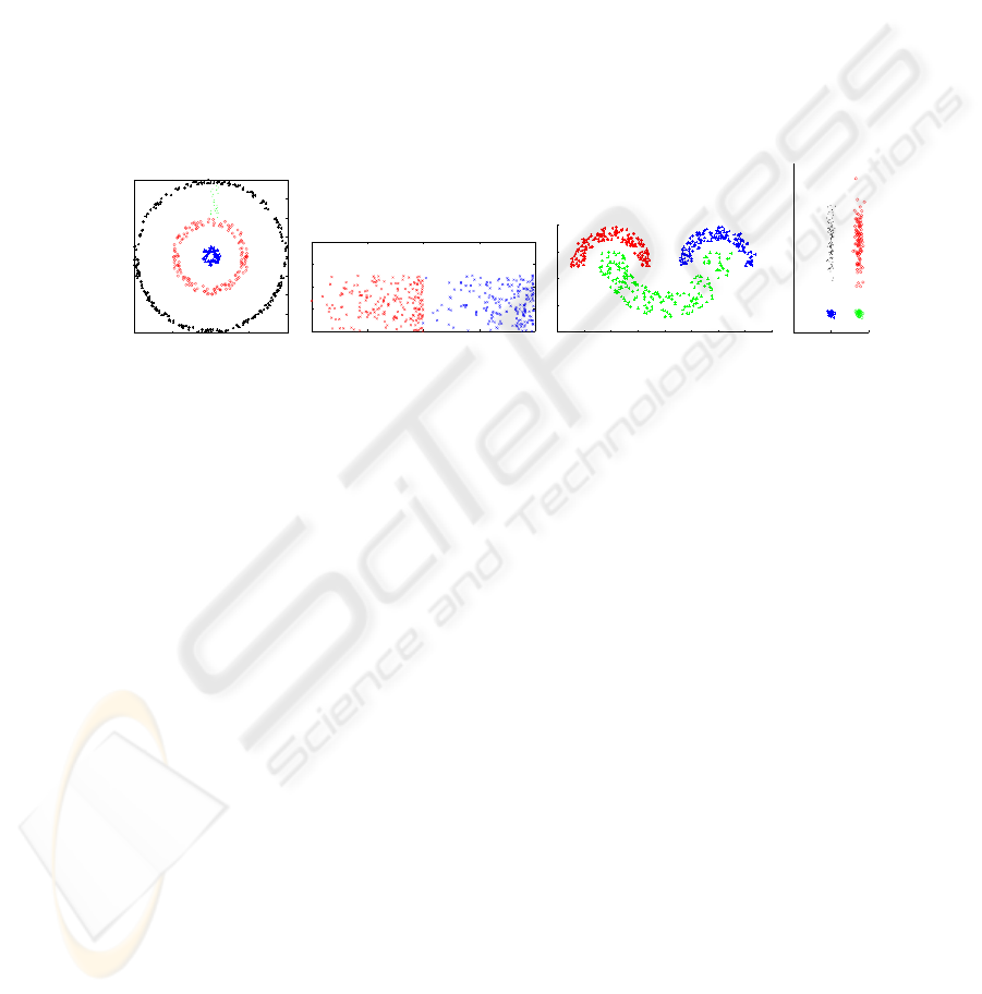
Synthetic Data Sets For simplicity of visualization, synthetic data sets con-
sist of 2-dimensional patterns. Data sets were generated in order to evaluate the
performance of the combination algorithms in a variety of situations, such as
arbitrary shaped clusters, distinct data sparseness in the feature space,well sep-
arated and touching clusters. Figure 1 plots these data sets. The Rings data set,
consists of 500 samples organized in 4 classes (with 25,75,150 and 250 patterns
each). The Bars data set is composed by 2 classes (200,200), the density of the
patterns increasing with increasing horizontal coordinate. The Half Rings data
set has 3 uniformly distributed classes (150-150-200) within half-ring envelops.
The Cigar data set has 4 classes (with 100,100,25 25 patterns each).
−2 −1 0 1 2
−2
−1.5
−1
−0.5
0
0.5
1
1.5
2
(a) Rings.
0 0.5 1 1.5 2
0
0.2
0.4
0.6
0.8
(b) Bars.
−8 −6 −4 −2 0 2 4 6 8
−6
−4
−2
0
2
(c) Half Rings.
−2 0 2
−5
−4
−3
−2
−1
0
1
2
3
4
(d) Cigar.
Fig. 1. Synthetic Data Sets.
Real Data Sets The first real application concerns DNA microarrays. The
yeast cell data consists of the fluctuations of the gene expression levels of over
6000 genes over two cell cycles. The available data set is restricted to the 384
genes (http://staff.washington.edu/kayee/model/) who’s expression level peak
at different time points corresponding to the 5 phases of the cell cycle. We used
the logarithm of the expression level and a ”standardized” version of the data
(with mean zero and variance 1) as suggested in [15]. The clustering process
should join the expression levels corresponding to the 5 phases of the cell cycles.
The second real data set, Handwritten Digits, is available at the UCI repos-
itory (http://www.ics.uci.edu/∼mlearn/MLRepository.html). From a total of
3823 available training samples (each with 64 features) we used a subset com-
posed by the first 100 samples of all the digits [12].
4.2 Combination of Clustering Ensembles Produced by K-Means
and Spectral clustering
To evaluate the performance of the combination methods, we will compare the
combined data partitions, P
∗
, with ground truth information, P
o
, obtained from
known labelling of the data. We will assume that the true number of clusters,
K, is known, being the number of clusters in P
∗
. We use the consistency index
proposed in [3] to assess the quality of a clustering, C
i
(P
∗
, P
o
); it is defined
227

as the fraction of shared samples in matching clusters of P
∗
and P
o
. When
data partitions have the same number of clusters, C
i
(P
∗
, P
o
) is equal to the
percentage of correct labelling.
EAC Graph Finite Mixture
Data Set K
i
SL CL AL WL Cent CSPA HGPA MCLA Max Mean STD L
Rings
Spectral
3 61.4 44.6 48.4 48.4 48.4 45.0 25.4 41.6 61.8 46.5 9.0 61.8
4 47.6 51.4 50.0 50.4 50.0 63.2 25.4 43.0 85.8 54.3 13.0 49.8
20 80.0 40.0 81.8 79.6 59.8 70.4 72.8 59.2 55.0 47.3 6.0 45.6
All 80.4 46.0 50.8 48.2 46.2 67.0 51.6 50.4 62.0 46.0 6.0 50.2
Kmeans All 85.6 40.0 44.6 59.4 51.0 47.8 67.2 61.2 60.60 50.30 8.00 59.4
Dist 58.8 36.8 34.0 43.4 43.6
Half Rings
Spectral
3 64.6 85.8 86.2 87.6 86.2 83.2 45.4 84.6 85.2 68.7 9.0 83.2
8 69.8 41.2 97.2 92.8 58.2 93.4 92.6 95.0 72.8 56.7 9.0 62.6
All 95.0 87.6 95.0 95.0 95.0 93.2 89.2 93.0 74.6 58.6 12.0 51.0
Kmeans All 99.8 38.2 95.0 95.0 51.6 93.4 95.0 93.8 56.60 46.30 6.00 56.6
Dist 95.0 72.0 73.4 73.6 73.6
Cigar
Spectral
4 100.0 100.0 100.0 100.0 100.0 71.2 34.4 100.0 100.0 88.8 11.0 100.0
5 100.0 61.6 100.0 100.0 100.0 70.8 41.2 73.6 100.0 81.8 9.0 100.0
8 100.0 61.6 100.0 70.4 79.6 70.0 70.4 66.8 72.8 59.4 8.0 58.8
All 100.0 100.0 100.0 100.0 100.0 70.4 74.8 63.2 54.0 44.8 7.0 44.4
Kmeans All 100.0 64.0 71.0 70.0 67.0 60.0 73.0 61.0 74.40 51.60 11.00 74.4
Dist 60.4 55.6 87.2 58.0 51.6
Bars
Spectral
2 96.8 96.8 96.8 96.5 96.8 99.0 50.0 96.8 97.0 96.7 0.3 96.8
15 99.5 55.0 99.5 99.5 55.8 99.2 97.0 99.5 80.5 62.9 10.0 80.5
All 98.8 97.5 97.5 98.8 97.5 97.8 98.8 98.8 75.5 59.4 8.0 75.5
Kmeans All 54.3 55.5 98.8 98.8 57.5 99.0 98.0 99.0 79.30 63.00 10.00 74.2
Dist 50.2 98.8 98.8 99.5 99.5
Log Yeast
Spectral
4 31.5 25.8 33.6 36.2 34.1 35.2 22.1 36.2 37.2 35.5 1.0 37.2
5 34.4 41.9 37.2 37.8 37.2 34.9 31.3 44.5 37.8 34.0 4.0 34.4
6 34.6 33.1 38.3 39.3 38.3 36.2 30.7 38.0 46.6 35.9 7.0 33.6
20 35.9 34.4 45.3 37.8 37.5 35.4 40.1 39.3 44.0 39.7 3.0 36.2
All 34.4 30.2 36.5 36.5 35.7 32.6 29.2 32.8 44.3 42.0 2.00 40.4
KMeans All 37.0 27.0 41.0 35.0 41.0 34.0 32.0 32.0 39.80 36.40 3.00 36.20
Dist 34.9 28.9 28.6 35.9 30.7
Std Yeast
Spectral
4 35.7 66.7 66.4 64.3 66.9 60.4 38.0 66.1 64.6 59.8 5.0 64.6
5 49.2 57.3 66.1 65.4 66.1 59.4 38.8 64.3 65.9 59.6 6.0 65.9
6 45.6 61.5 68.2 65.4 68.2 56.5 37.2 67.2 63.8 57.8 5.0 60.9
20 36.2 43.2 62.8 52.3 39.3 55.5 56.5 59.1 60.9 54.3 6.0 57.0
All 44.8 65.6 65.9 65.4 65.1 56.8 59.4 58.9 64.1 52.8 12.0 64.1
KMeans All 48.0 54.0 67.0 56.0 45.0 53.0 57.0 54.0 51.60 45.20 8.00 39.30
Dist 36.2 66.7 65.9 66.9 57.8
Optical
Spectral
9 60.5 79.0 77.3 84.3 77.3 79.5 35.2 79.5 77.1 65.3 9.0 77.1
10 70.0 77.3 77.6 84.5 77.6 80.5 33.4 84.5 75.6 69.7 6.0 67.9
15 72.2 53.0 72.2 88.3 73.8 86.3 52.7 78.1 75.9 67.4 8.0 75.9
All 60.4 75.0 79.1 87.3 79.1 88.1 45.4 77.1 72.6 67.8 4.0 72.6
Kmeans All 40.0 51.0 79.0 80.0 71.0 84.0 78.0 88.0 64.00 57.90 4.00 54.30
Dist 10.6 54.1 75.7 74.8 10.6
Table 1. Combination Results - C
i
(P
∗
, P
o
) - for Spectral and K-means Clus-
tering Ensembles. Best results for each clustering ensemble are represented in
bold style.
Table 1 shows the C
i
(P
∗
, P
o
) index for spectral and K-means clustering
ensembles with both synthetic and real data sets (see first column). In this
table, rows are grouped by clustering ensemble construction method (second
column). Rows corresponding to Spectral Clustering Ensembles, with numerical
labels in the K
i
column indicate that the clustering ensemble has only par-
titions with K
i
clusters (method (i) in section 2.1). For each K, a clustering
ensemble with N = 22 data partitions was produced by assigning σ values be-
tween 0.08 and 0.5, with increments of 0.02 (schematically described by the
notation [0.08:0.02:0.5]). We have tested with K taking all the values in the set
K = {2, 3, 4, 5, 6, 7, 8, 9, 10, 15, 20}; due to space limitations, only a small number
of experimental results are presented. Rows corresponding to Spectral Clustering
Ensembles, with the label ”All” (method (ii) in section 2.1) correspond to the
union of all the partitions produced by method (i) with K taking all the values
228

in the set K (N = 242). For the K-means ensemble the row ”All” represents the
results obtained with N=200, and K randomly chosen in the set {10, . . . , 30}.
Finally the rows ”Dist” represent the results obtained by each of the hierarchical
clustering methods directly applied to the Euclidean distance matrix between
objects in the original feature space.
Columns are grouped by combination method. Corresponding to the EAC
method, columns with titles ”SL”, ”CL”, ”AL”, ”WL” and ”Cent” represent the
methods of extraction of the final data partition, respectively: Single Link, Com-
plete link, Average link, Wards Link and Centroid Linkage. The Graph based
strategy has three columns corresponding to the heuristics ”CSPA”, ”HGPA”
and ”MCLA”. Computation of these results used the Matlab implementation
made available at (http://strehl.com). The last method - Finite Mixture - is
characterize by columns ”Max”, ”Mean, ”STD” and ”L”, representing the max-
imum, the mean, and standard deviation of the consistency index over 10 runs of
EM algorithm (for the real data sets only 5 runs were used); column L represents
the best run using the established criteria (likelihood).
From the analysis of table 1 we see that none of the methods is a clear winner
(each combination method produces best results at least once). Observation of
the clusters structure help to enlighten which method is more suitable for each
situation. When dealing with arbitrary shaped, well separated clusters, such as
in the Half Rings and the Cigar data sets, the EAC method performed better
than the others; the superiority of the SL variation of the EAC method is here
particularly evident when comparing results with clustering ensembles produced
by the K-means algorithm, as the spectral clustering algorithm maps the original
feature space to another space where clusters are more compactly represented,
and therefore clustering algorithms favoring compacticity should work well. In
situations of touching clusters (Rings and Bars), the Graph based heuristics have
a performance similar to EAC. In the real data sets the performance is very good
compared with the results presented in [12], where for Optical Digits the best
result was about 20% of clustering error, and with the combination of clusterings
the best error rate achieved is about 10%. For the log-normalized yeast cell data
the results were worst than in [12], where clustering error is about 40% compared
with the 55% in the present work. Finally for the standardized yeast cell data
in [12] the clustering error was 35%, which is comparable to the best error rate
present in table 1.
Comparison of K-means based and spectral clustering based combination re-
sults show that the combination of clustering ensembles produced by the spectral
clustering algorithm leads, in general, to better data partitions (at the expense of
a higher computational burden); when dealing with well separated clusters, both
methods of constructing the clustering ensemble lead to comparable results, the
K-means approach being a more adequate choice due to its low computational
complexity. Application of the hierarchical clustering algorithms directly to the
Euclidean distances between patterns lead, most of the times, to the po orest
performances observed.
229
0 20 40 60 80 100 120 140
0.35
0.4
0.45
0.5
0.55
0.6
0.65
0.7
0.75
0.8
0.85
EAC
Number of Partitions
C
i
single
complete
average
ward
centroid
(a) EAC.
0 20 40 60 80 100 120 140
0.4
0.45
0.5
0.55
0.6
0.65
0.7
0.75
Strehl & EM
Number of Partitions
C
i
CSPA
HGPA
MCLA
EM
(b) HyperGraph and Finite Mixture.
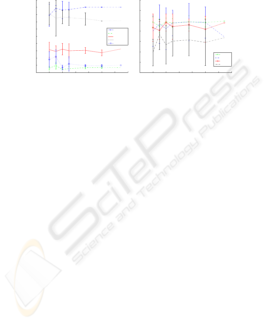
Fig. 2. Evolution of mean values and standard deviation of C
i
(P
∗
, P
o
) as a function
of N , the number of partitions in the clustering ensemble, for the Rings data set; the
clustering ensemble was created using the spectral clustering algorithm with K = 15
and σ =[0.08:0.01:0.99 1:.25:10].
Another interesting comparison between the methods concerns the rate of
convergence and stability of the combination solutions as a function of N, the car-
dinality of the clustering ensemble. We have observed that the EAC method leads
to better convergence curves, the variance of the consistency index C
i
(P
∗
, P
o
),
as computed over 10 repetitions of the combination experiment, decreasing to
zero, a value that is achieved with N < 200 in all data sets under study. Figure
2 illustrates the results of the C
i
(P
∗
, P
o
) for the the Rings data set, using spec-
tral clustering with K = 15, and randomly picking partitions obtained with σ
in set [0.08:0.01:0.99 1:.25:10]. As the number of partitions grows, the standard
deviation of C
i
(P
∗
, P
o
) for the EAC methods diminish, the combined partition
converging to a unique solution (null variance) with N < 120; the other com-
bination methods, however, with the exception of CSPA, present not so stable
solutions, exhibiting large variances of results over the entire interval for N .
4.3 Selection of the Combination Method
We have empirically demonstrated in the previous section that none of the com-
bination methods under study proves to be the best for all situations, results
depending on the data sets, and on the way of producing the clustering ensemble.
Strehl and Gosh [4] proposed to use the average normalized mutual information
- ANMI(P
∗
, P) (see section 3.2) - as criteria for selecting among the combina-
tion results produced by different combination strategies. We now compare the
several methods based on this consensus measure, and investigate its usefulness
for the selection of the combination method.
Table 2 presents the values of AN M I(P
∗
, P) for the data sets and combi-
nation methods in correspondence with table 1, exception made for the Finite
230

Mixture column that corresponds to column L in table 1. It is easy to see that
none of the methods gives overall best consensus with the clustering ensemble:
highest ANMI(P
∗
, P) values are distributed along all columns in this table.
Data Set K
i
SL CL AL WL Cent CSPA HGPA MCLA Finite Mixture (L)
Rings
3 0.448 0.609 0.606 0.607 0.606 0.517 0.003 0.602 0.605
4 0.655 0.789 0.798 0.799 0.798 0.610 0.007 0.740 0.717
20 0.553 0.228 0.621 0.513 0.363 0.619 0.631 0.604 0.573
All 0.511 0.553 0.630 0.632 0.635 0.511 0.483 0.629 0.311
kmeans 0.5693 0.3666 0.5791 0.4910 0.2943 0.5693 0.5840 0.5768 0.3954
Half Rings
3 0.666 0.843 0.842 0.833 0.842 0.831 0.187 0.842 0.844
8 0.392 0.364 0.598 0.579 0.403 0.581 0.594 0.603 0.530
All 0.609 0.610 0.609 0.609 0.609 0.599 0.608 0.610 0.524
kmeans 0.5234 0.2185 0.5380 0.5380 0.2323 0.5201 0.5380 0.5277 0.2370
Cigar
4 0.994 0.994 0.994 0.994 0.994 0.669 0.120 0.994 0.994
5 0.908 0.641 0.908 0.908 0.908 0.693 0.177 0.814 0.908
8 0.753 0.519 0.753 0.777 0.678 0.704 0.722 0.762 0.723
All 0.750 0.750 0.750 0.750 0.750 0.609 0.615 0.675 0.451
kmeans 0.5941 0.5412 0.6401 0.6400 0.4553 0.6115 0.6249 0.5962 0.4308
Bars
2 0.974 0.974 0.974 0.969 0.974 0.852 <0.001 0.974 0.974
15 0.395 0.094 0.395 0.395 0.144 0.389 0.394 0.395 0.338
All 0.543 0.545 0.545 0.543 0.545 0.516 0.543 0.543 0.236
kmeans 0.0817 0.1089 0.3816 0.3816 0.1462 0.3661 0.3812 0.3816 0.2508
Log Yeast
4 0.052 0.615 0.662 0.652 0.662 0.565 0.422 0.659 0.645
5 0.050 0.596 0.590 0.604 0.614 0.558 0.487 0.576 0.543
6 0.049 0.521 0.600 0.580 0.560 0.545 0.537 0.561 0.536
20 0.341 0.349 0.562 0.565 0.200 0.531 0.551 0.544 0.483
All 0.064 0.503 0.537 0.539 0.494 0.520 0.428 0.525 0.351
kmeans 0.3165 0.4192 0.6143 0.6041 0.3041 0.6011 0.6001 0.6065 0.3697
Std Yeast
2 0.492 0.632 0.753 0.757 0.755 0.693 0.287 0.753 0.721
3 0.029 0.633 0.720 0.710 0.722 0.664 0.304 0.721 0.670
4 0.345 0.630 0.708 0.707 0.707 0.654 0.391 0.660 0.687
5 0.062 0.202 0.590 0.570 0.188 0.571 0.566 0.565 0.511
All 0.332 0.625 0.659 0.655 0.657 0.616 0.511 0.623 0.523
kmeans 0.4202 0.4720 0.6304 0.6489 0.3595 0.6325 0.6487 0.6386 0.4633
Optical
9 0.844 0.921 0.944 0.933 0.944 0.867 0.425 0.910 0.885
10 0.829 0.928 0.937 0.929 0.937 0.855 0.388 0.928 0.890
15 0.878 0.783 0.907 0.921 0.883 0.855 0.590 0.878 0.861
All 0.766 0.758 0.754 0.741 0.754 0.699 0.463 0.595
kmeans 0.4803 0.6144 0.7850 0.7819 0.7680 0.7567 0.7338 0.7782 0.6065
Table 2. Values of the consensus function AN M I(P
∗
, P) for the data sets and
situations in table 1.
Comparison of best results according to the consistency measure with ground
truth information, C
i
(P
∗
, P
o
), in table 1 with the consensus measure with the
clustering ensemble, ANM I(P
∗
, P), in table 2 leads to the conclusion that there
is no correlation between these two measures; therefore, the mutual information
based consensus function is not suitable for the selection of the best performing
method in each situation.
5 Conclusions
In this work we addressed the problem of combining multiple data partitions in
the context of spectral clustering and k-means clustering. Clustering ensembles
were either produced by using the K-means algorithm or the spectral cluster-
ing algorithm by Ng et al [11], with different parameter values and/or different
initializations. Three different combination strategies found in the literature,
namely evidence accumulation clustering, graph based combination and maxi-
mum likelihood combination (finite mixture model), were compared and ana-
lyzed empirically. Test data sets consisted both on synthetic data, illustrating
different cluster structures, and real application data. For each data set, and each
231

clustering ensemble, the several combination algorithms, and variants herein pro-
posed, were applied in order to obtain the combined data partition P
∗
. Using
known labelling of the data - ideal partition P
o
- as ground truth information, a
consistency index between the combined data partition, P
∗
, and P
o
(C
i
(P
∗
, P
o
))
was computed. Comparison of the several combination methods using this con-
sistency index has shown that there is no best method for all situations, results
depending on the data sets and on the way of building the clustering ensembles.
The finite mixture model seems to be more appropriate for situations with clus-
tering ensembles with a few number of partitions where the number of clusters in
each partition is near the true number of clusters. The other methods (EAC and
Graph based) seem more robust and can better handle most situations. Analy-
sis of the variance of the consistency measure, computed over multiple runs of
the experiments, has shown that the evidence accumulation strategy leads to
more stable results, converging to a unique combination solution (null variance
of C
i
(P
∗
, P
o
)) when the cardinality of the clustering ensemble, N, is sufficiently
large, typically with N < 200; the other techniques exhibit, most of the times,
a large variance for the consistency index. The problem of selecting amongst
the combination results was also addressed using the mutual information based
consensus measure proposed by Strehl and Gosh [4], measuring the consensus be-
tween the combined partition and the clustering ensemble. Experimental results
demonstrated that this measure is not adequate for selecting the best perform-
ing method, as there is no correspondence between best consensus values and
consistency with ground truth information.
Ongoing work include the investigation of criteria for the comparison and
selection of best combination techniques.
References
1. J. Kittler, M. Hatef, R. Duin, and J. Matas. On combining classifiers. IEEE Trans.
Pattern Analysis and Machine Intelligence, 20(3):226–239, 2000.
2. Fabio Roli and Josef Kittler. Fusion of multiple classifiers. In Information Fusion,
volume 3, page 243, 2002.
3. A. Fred. Finding consistent clusters in data partitions. In Josef Kittler and
Fabio Roli, editors, Multiple Classifier Systems, volume LNCS 2096, pages 309–
318. Springer, 2001.
4. A. Strehl and J. Ghosh. Cluster ensembles - a knoledge reuse framework for com-
bining multiple partitions. Journal of Machine Learning Research 3, 2002.
5. B. Park and H. Kargupta. Data Mining Handbook, chapter Distributed Data Min-
ing. Lawrence Erlbaum Associates, 2003.
6. A. Fred and A.K. Jain. Data clustering using evidence accumulation. In Proc. of
the 16th Int’l Conference on Pattern Recognition, pages 276–280, 2002.
7. X. Z. Fern and C.E. Brodley. Random projection for high dimensional data cluster-
ing: A cluster ensemble approach. In Proceedings of 20th International Conference
on Machine learning (ICML2003), 2003.
8. A. Topchy, A.K. Jain, and W. Punch. A mixture model of clustering ensembles.
In Proceedings SIAM Conf. on Data Mining, April 2004. in press.
232

9. Erik L. Johnson and Hillol Kargupta. Collective, hierarchical clustering from dis-
tributed, heterogeneous data. In Large-Scale Parallel Data Mining, pages 221–244,
1999.
10. E. Dimitriadou, A. Weingessel, and K. Hornik. A voting-merging clustering al-
gorithm. In SFB, editor, FuzzyNeuro Systems ’99, volume Adaptive Information
Systems and Modeling in Economics and Management Science, April 1999.
11. A.Y. Ng, M.I. Jordan, and Y. Weiss. On spectral clustering: Analysis and an
algorithm. In S. Becker T. G. Dietterich and Z. Ghahramani, editors, Advances in
Neural Information Processing Systems 14, Cambridge, MA, 2002.
12. D. Verma and M. Meila. A comparision of spectral clustering algorithms. Technical
rep ort, UW CSE Technical report, 2003.
13. G. Karypis and V. Kumar. Multilevel algorithms for multi-constraint graph par-
titioning. In Proceedings of the 10th Supercomputing Conference, 1998.
14. G.Karypis, R.Aggarwal, V.Kumar, and S.Shekhar. Multilevel hypergraph parti-
tioning: Applications in vlsi domain. In Proc. Design Automation Conf., 1997.
15. A. Raftery K. Yeung, C.Fraley and W.Ruzzo. Model-based clustering and data
transformation for gene expression data. Technical Report UW-CSE-01-04-02,
Dept. of Computer Science and Engineering, University of Washington, 2001.
233
