
REAL-TIME MODELLING OF WOOD DRYING SYSTEMS
Learning from Experiment and Theory
Stanislaw Tarasiewicz
Department of Mechanical Engineering, Laval Université, Québec, Canada
Belkacem Kada
Department of Mechanical Engineering, Laval Université, Québec, Canada
Keywords: Mathematical modelling, numerical simulation, com
puter model, on-line identification, operating functions,
state variables.
Abstract: Predictive control in a wood drying systems is still at an early stage, because of the difficulties with the
estimating a temporal moisture distribution for the whole dried lumber. Therefore, based on the dry and
wet-bulb temperatures as the state variables the temporal moisture distribution in kiln-dried lumber is
determined from numerical solutions of mathematical model for the wood drying systems. This computer
model is represented by a set of several partial nonlinear differential equations coupled with the operating
functions and a set of several calculating algorithms. The accuracy of the model solutions in a real-time
calculation is evaluated by the on-line identification of the operating functions that represent both the
system parameters (heat transfer coefficients, thermal conductivity, heat capacity etc) and selected state
variables (air temperature, humidity, velocity etc).
1 INTRODUCTION
Though drying of lumber in the wood kiln is a
simultaneous heat and mass transfer process, the
temporal mass changes are less pronounced than the
heat (energy) changes because of high latent heat of
water and thus prevailing thermal effects during
evaporation and condensation. Therefore, the
classical approach to drying as water removal can
conveniently be regarded as a heat exchange process
between the drying gas (air) and the solid material
(lumber). Because the lumber boards for drying are
stacked into piles and several piles are placed in the
kiln, the kiln and its load is considered as a wood
drying system (WDS). Typically, the WDS is treated
as a lumped-parameter system, and thus its dynamic
behaviour can be described by the input-output
transfer functions. However, establishing a dynamic
mathematical model to be practical enough for
control applications requires so many simplifying
assumptions that the model hardly reflects the real
situation. A compromise between the complex but
adequate model and its simplification can be
obtained when taking advantage of the measured
temperature profiles in a given system, and solving
numerically the partial differential equations by
decomposing the solutions into the so-called
regulated variables at the defined boundary
conditions. The accuracy of these solutions has to be
evaluated by the on-line identification (OLI) system.
In return, the on-line identification, as a supporting
tool for computer modelling, allows determination
of the temperature profiles across the kiln as to avoid
conditions that may lead to lumber degradation.
2 MATHEMATICAL
FORMULATIONS
The model is based on the well established drying
mechanism for lumber. During the pre-heating
period, the temperature of stacked lumber is
equilibrated to the air temperature by heating at the
controlled rate to prevent condensation of water
vapour. At the end of this period, the moisture
content (MC) of lumber is assumed uniform. During
the constant rate period, the vapour pressure at the
lumber surface is equal to the saturated vapour
pressure, and the surface temperature approaches the
wet-bulb temperature.
132
Tarasiewicz S. and Kada B. (2005).
REAL-TIME MODELLING OF WOOD DRYING SYSTEMS - Learning from Experiment and Theory.
In Proceedings of the Second International Conference on Informatics in Control, Automation and Robotics - Signal Processing, Systems Modeling and
Control, pages 132-136
DOI: 10.5220/0001159601320136
Copyright
c
SciTePress
If the external conditions are constant, then the
drying rate is also constant, down to the fibre
saturation point (FSP) of about 30 % wb. Below the
FSP, the drying rate decays exponentially whereas
the surface temperature increases progressively
towards the air temperature. The mathematical
model for drying lumber that leads to temperature
distribution along the kiln can be obtained by using
the control volume method (Kada, B. and
Tarasiewicz, S., 2004, and Tarasiewicz, S., 1984,
Tarasiewicz, S. et al., 2000 and Tarasiewicz, S. et
al., 1982). The moving control volume shown in Fig.
1 is selected as to comprise the lumber and the air
gap. Normally, the control volume covers the length
of the lumber board (L
z
). However, it can be reduced
to the incremental length (dz) to avoid local defects
such as cracks or knots. The overall mathematical
model for the WDS comprises the following
equations (another form of the model is given in
Appendix):
(1)
where: z( x, t ) = [ M( x, t ) T( x, t ) ]
T
is the vector
of distributed state variables (MC and wood
temperature ); u( x, t ) = [ T
a
( x, t ) v
a
( x, t ) ]
T
is the
vector of distributed control variables, namely air
temperature and air velocity (air mass displacement),
and A
wi
, B
w
, A
ai
, B
a
are modified operating functions
for i = 0, 1, 2, 3, and A
w3
is proportional to F
10
(see
Appendix)
.
The initial and boundary conditions are
(2)
(3)
where: D
wi
, D
ai
, for i = 0 - 3 (number of the
heating/drying zones), R
w
, R
a
are the
complementary OFs, and
x = x, for 0< x < L (L =
L
x1
+ L
x2
+ … + L
xn
is the total length of the n
lumber piles).
This mathematical model follows the drying
mechanism as it reflects the dynamics of moisture
change during drying. The operating functions can
be further improved through calculation procedures
of all distributed variables (state variables and
control variables), and compared with either the
target values of the distributed state profiles or with
the measured values, if possible.
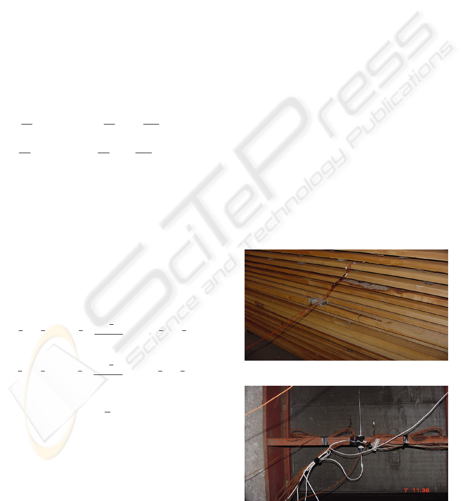
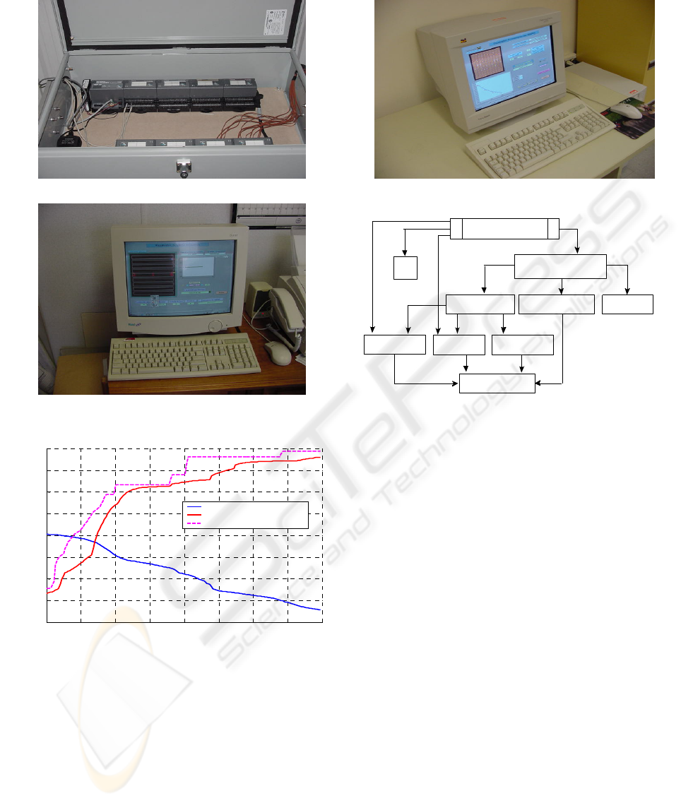
3 INSTRUMENTATION AND
EXPERIMENTAL
IDENTIFICATIONS
The experiments on on-line identification were
performed in a typical wood kiln equipped with the
data acquisition system (see Fig. 1a, 1b, 1c, 1d).
The experimental reconstructed profiles of the state
distributed variables, for this system, are plotted in
Figure 1e.
To validate the distributed state values calculated
from the proposed mathematical model(see Fig. 2a),
the operating functions in Eq. 1 (and Eqs. 5 through
7 in Appendix) should be decomposed into two
independent functions either by using the
hierarchical structure (see Fig. 2b) or by using the
techniques of separated variables (Kada, B. and
Tarasiewicz, S., 2004, and Tarasiewicz, S., 1994):
OF
i
( x, t.) = f
i
( x ) × g
i
( t ) for i = 1,…, N (4)
where: f
i
(x) are the distributed functions
proportional to the mean parameters under
consideration, g
i
(t) are the dynamic functions of
physical parameters, and N is the number of the
defined OFs.
a)
b)
⎪
⎩
⎪
⎪
⎨
∂
∂
∂
t
+
∂
∂
+
∂
∂
+=
∂
∂
+
∂
+
∂
+=
∂
zB
u
A
u
AuA
u
A
uB
z
A
z
AzA
z
A
.
x
.
x
.
t
.
.
x
.
x
..
a
2
2
3a2a1a0a
w
2
2
3w2w1w0w
=
xx
xx
u
zz
⎪
⎧
⎨
= u
)()0,(
)()0,(
0
0
⎩
⎧
⎪
⎪
⎨
⎩
⎪
⎪
⎧
=+
=+
),().,(
),(
).,(),().,(
),().,(
),(
).,(),().,(
10
10
txtx
x
tx
txtxtx
txtx
x
tx
txtxtx
aaa
www
zR
u
DuD
uR
z
DzD
∂
∂
∂
∂
REAL-TIME MODELLING OF WOOD DRYING SYSTEMS - Learning from Experiment and Theory
133
c)
d)
e)
Figure 1: Data acquisition system; a) sensor locations in
lumber; b) sensor locations in air; c) transducers; d)
microcomputer-based network (implemented in the
industry) as a Reconstruction System (RS) of the
distributed state variables; e) reconstructed profiles of the
state distributed variables for the WDS (see Fig. 1d)
a)
v)
csaa t
= f(T
,T
,v
,W,D
D= f(k
t aapa
,
ρ
,c )
k= f(T
a
db
,T
wb
)
ρ
a
= f(T
db
,T
wb
)
c
pa
=f(T
db
)
F
6
= f(T
db
,T
wb
,v
a
)
v
a
=
measurab le
F
6capa6
= f(v ,
ρ
,c ,C )
W = .co n s t
C
6
b)
Figure 2: Microcomputer-based network
0 5 10 15 20 25 30 35 40
10
20
30
40
50
60
70
80
90
time [Day]
Moisture [%] - Temperature [°C]
Mean values of moisture and temperature
Moisture content of Wood
Temperature of Wood
Temperature of Air
Where: a) Numerical Calculator (NC) to
estimating the distributed state variables
(implemented in the Complex Automation and
Mechatronic Laboratory (LACM)); b) hierarchical
structure of the sample operating function and its
physical parameters (for details, see Tarasiewicz, S.
et al., 2000); the C
6
is a tuning parameter.
The communication between NC and RS (see
Fig.1d) were performed via Internet Network in real-
time.
From the above subdivision of this operating
function one can conclude that its calibrated
parameters are the dry and wet-bulb temperatures
(T
db,
and T
wb
) and air velocity (v
a
).
Characteristically, for all operating functions it is
possible to apply the same calibration procedure as
shown in Fig. 2b, and the same calibrated
parameters, namely T
db
, T
wb
and v
a
.
To complete the validation (calculation) procedures,
the Runge-Kutta method has been used. The
software has been written in the C++ language, and
the results of computations have been shown in Lab
view windows (c.f., Figs. 3a, 3b, and 4).
ICINCO 2005 - SIGNAL PROCESSING, SYSTEMS MODELING AND CONTROL
134
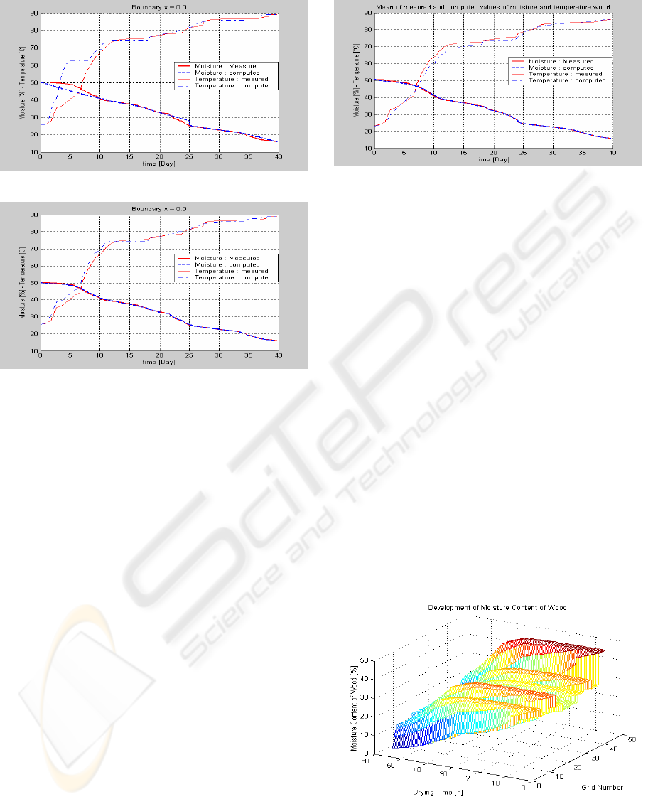
a)
b)
Figure 3: Calculated profiles of the state distributed
variables for the WDS; a) initial tuning parameters; b)
tuning parameters are the air temperature function (for
comparing, see Fig. 1e)
From the preliminary simulation tests shown in
Figure 3a it was clear the operating functions in
boundary conditions (Eq. 3) have to be modified.
Thus, in the subsequent simulation tests, some
physical properties of the drying lumber have been
determined, and numerical results obtained for these
boundary conditions are plotted in Figure 3b.
The proposed mathematical model (given either by
Eq. 1 or Eqs. 5-7 with the admissible numerical
values of all OFs determined by using the proposed
algorithm (Tarasiewicz, S., et al., 2000, and
Tarasiewicz, S., et al., 1994)), was validated and the
results are plotted in Figures 3 and 5
Figure 4: Evaluation and comparison of the state
distributed variables inside the WDS ( see Fig. 1e)
.
From these Figures it is evident that the numerical
solution of the mathematical models for the WDS
can adequately estimate (predict) the dynamic
evolution of the distributed state variables.
4 SUMMARY
Using the calculated profile with the calibrated OFs
(see Fig. 3b and Fig. 4) for the distributed air gap
temperature (T
a
), and kiln temperatures (T
db
and
T
wb
) it is possible to estimate the distributed
moisture content of lumber during drying (see Fig.
5). Also, by using the estimated profile of the MC
with the calibrated OFs (Fig. 4) for the WDS it is
possible to predict the distributed control variables
for the air temperature in the WDS.
The fact that computation time taking by the NC is
very short or much shorter as compared to the
reconstruction time taking by the RS confirms that
the numerical calculation can be utilized in a
predictive control structure.
Figure 5: Evolution of the moisture content in the whole
dried lumber for different values of the initial MC, and for
each piece of wood
REAL-TIME MODELLING OF WOOD DRYING SYSTEMS - Learning from Experiment and Theory
135

Because of system complexity, the control structure
has to be subdivided into a multilevel hierarchical
structure (Tarasiewicz, S., et al., 2000, and
Tarasiewicz, S., et al., 1994). Further, the predicted
profiles of the MC and air temperature would allow
building design of industrial controllers providing
real time control of the wood drying systems.
ACKKNOWLEDGEMENTS
This research was supported by the Natural Sciences
and Engineering Research Council of Canada (
CRSNG, PPT # 66700 ).
REFERENCES
Kada, B. and Tarasiewicz, S. 2004. Analysis and
identification of distributed parameter model for wood
drying systems ’’. Drying Technology, 22(5): 933–
946.
Tarasiewicz, S. 1984. Identification of an anode – baking
process in the ring furnace. Trans. Society for
Computer Simulation, 1(2): 117–132.
Tarasiewicz, S., Ding, F., Kudra, T. Mrozek, Z. 2000. Fast
and slow generation of a multilevel control for the
wood drying process. Drying Technology, 18(8):
1709–1735.
Tarasiewicz, S., Bui, R.T. and Charette, A. 1982. A
computer model for the cement kiln. IEEE Trans.
Industry Applications, IA – 18(4): 424–430.
Tarasiewicz, S., Gille, J-C., Léger, F. and Vidal, P. 1994.
Modelling and simulation of complex mechanical
systems with applications to a steam – generating
system. Part 1 and 2. Int. J. Systems Sci., 25(12):
2394–2402, Part 1, and 25(12): 2403–2416, Part 2
.
APPENDIX
The alternative form of the mathematical model is
give by the following equations:
⎥
⎥
⎥
⎥
⎥
⎦
⎤
⎢
⎢
⎢
⎢
⎢
⎣
⎡
∂
∂
+
∂
∂
∂
∂
+
∂
∂
+
∂
∂
∂
∂
+
∂
∂
−=
∂
∂
),(
),(
),(
),(
),(
),(
),(
),(
),(
),(
),(
),(
1211
2
2
11
10
2
2
10
12
txM
t
txF
x
txT
x
txF
x
txT
txF
x
txM
x
txF
x
txM
txF
t
txM
txF
[]
⎥
⎥
⎥
⎥
⎥
⎥
⎥
⎥
⎥
⎥
⎥
⎦
⎤
⎢
⎢
⎢
⎢
⎢
⎢
⎢
⎢
⎢
⎢
⎢
⎣
⎡
−
+
∂
∂
+
∂
∂
−
∂
∂
∂
∂
+
∂
∂
=
∂
∂
−
∂
∂
),(),(),(
),(
),(
),(
),(
),(
),(
),(
),(
),(
),(
),(
),(
7
98
5
2
2
5
98
txTtxTtxF
txM
t
txF
txT
t
txF
x
txT
x
txF
x
txT
txF
t
txM
txF
t
txT
txF
a
⎥
⎥
⎥
⎥
⎦
⎤
⎢
⎢
⎢
⎢
⎣
⎡
Π+−
∂
∂
+
∂
∂
+
⎥
⎦
⎤
⎢
⎣
⎡
∂
∂
+
∂
∂
−
∂
∂
−
=
∂
∂
τ
gtxFtxP
x
txF
x
txP
txF
txv
x
txv
txF
t
txF
txv
x
txF
t
txv
txF
a
a
a
a
),(),(
),(
),(
),(
),(
),(
),(
),(
),(
),(
),(
),(
3
2
2
1
1
2
1
1
Where: F
j
for j = 1,…,12 are the operating functions,
P is the total pressure in the air gap, П is the gap
perimeter available to air flow, τ is the shear stress
induced in wood by moisture and temperature
gradients.
ICINCO 2005 - SIGNAL PROCESSING, SYSTEMS MODELING AND CONTROL
136
