SYSTEMATIC APPROACH TO MODEL-BASED DATA SURVEY

Ari Isokangas, Mika Ruusunen and Kauko Leiviskä

University of Oulu, P.O.Box 4300, 90014 University of Oulu, Finland

Keywords: Identification, Input selection, Characterisation, Model construction, Process control.

Abstract: A framework for surveying multivariate process data is prese

nted. Systematic procedure utilises linear

model candidates constructed in sliding data windows of varying length, to determine the usefulness of data

segments for process identification. The discussed survey approach was applied to an industrial wood

debarking data, enabling the study of process variables and conditions affecting the wood losses. In

addition, main process interactions and delays were easily discovered from the structures of the interpretable

linear model candidates. The analysis can thus provide valuable information also for process modelling and

control.

1 INTRODUCTION

Information retrieval from data is the first and

crucial step in order to obtain knowledge for process

identification. At this stage, one wants to point out

the usefulness and possible problem areas of data

(Pyle, 1999). This, in turn, requires that a

representative sample of the population is available,

for example, applying the design of experiments

(DOE). However, industrial data sets are often in

large databases incorporating all the unmeasured

disturbances and changing operating conditions. In

these cases, data analysis via trial and error can be

laborious. This paper describes an approach to

survey data with a systematic model-based

procedure.

A typical example of process d

ata that is difficult

to analyse, is data from the wood debarking process

in pulp and paper mills. There the costs of raw

material play an important role in the plant

economy. In the debarking process, 1-3% of raw

material goes as wood losses to the combustion

process with bark. The analysis of process and

determining the process parameters to minimise

wood losses may result in annual savings of

hundreds of thousands of euros.

Isokangas and Leiviskä (2005) modelled wood

sses of drum debarking without any special

emphasis on training data selection. Näsi et al.

(2001) used data clustering, but in both cases

analysis was not very successful. It was concluded

that this was partially due to inaccurate and

insufficient measurements of the debarking drum.

There was not, for example, any measurement for

the quality of raw material, which had a strong effect

on the process state. Also, wood loss data contained

a lot of process malfunctions and unmeasured

changes in operation conditions. The selection of

information rich data for modelling is important and

it can only be obtained with a proper data survey. In

this context, data survey means identifying general

properties of process relationships in data, leading to

the preliminary analysis of data for modelling.

There are studies concerning the length of

raining data to the performance of models.

Correctly selected training data incorporates

essential information about the phenomenon to be

modelled and models constructed with such data

worked well (Anctil, Perrin & Andréassian, 2004;

Kocjančič & Zupan, 2000). In this view, the main

idea of the presented approach is the procedure to

systematically search for information rich data

segments. For this purpose, it uses sliding windows

across a data set and varying window sizes. Locally

focused data analysis with windowing makes it also

possible to use linear techniques.

There are also many reported model structure

dentification methods, for example sliding data

window approach (Luo & Billings, 1995), fuzzy

cluster analysis (Šindelář, 2004; Abonyi, Babuška &

Feil, 2003), a modal symbolic classifier (Prudêncio,

Ludermir & de Carvalho, 2004), combined forward

and exhaustive search (Mendes & Billings, 2001),

including partly automated data pre-processing and

Isokangas A., Ruusunen M. and Leiviskä K. (2005).

SYSTEMATIC APPROACH TO MODEL-BASED DATA SURVEY.

In Proceedings of the Second International Conference on Informatics in Control, Automation and Robotics - Signal Processing, Systems Modeling and

Control, pages 60-65

DOI: 10.5220/0001165600600065

 SciTePress

identification method (Simon, Schoukens & Rolain,

2000). Other authors report also studies utilising

self-organising networks (Linkens & Chen, 1999)

and fuzzy algorithm for model structure

identification (Sugeno & Kang, 1988).

Abovementioned investigations have their focus

mainly on the automatic model input, order or

parameter selection. Unfortunately, only a few

researches deal with systematic data survey, for

example in the form of entropic analysis (Pyle,

1999), which covers issues needed for process

identification in all respects.

The approach in this paper intends to combine

necessary aspects for systematic data survey,

namely: providing easily interpretable results

without the need for complex pre-processing, and

systemising search of representative process

conditions in large databases. The method constructs

automatically linear dynamic model candidates,

from all available input combinations in every data

window examined. The final analysis concerns then

with the model structure properties of the best

candidate models. The performance assessment of

the models uses the root mean square error (RMSE)

values, correlation coefficients and the visual

appearance of the model behaviour.

The following sections introduce the framework

for model-based data survey and apply it to wood

loss data from a pulp mill. The paper concludes with

the analysis and discussion of the results

2 MODEL-BASED DATA SURVEY

APPROACH

2.1 Overview

The aim of the discussed data survey procedure is to

find interactions between variables from large

datasets. This occurs systematically by constructing

simple dynamic model candidates with complete

input combinations for data segments of varying and

sliding window size. The final analysis goes on

according to the model structure properties of the

best candidate models.

Linear model structure was chosen as a

candidate. Model simplicity guarantees the

modelling efficiency, because of the great number of

constructed and tested models. The theory of

estimating model parameters is well defined in the

literature (see Ljung, 1999; Söderström & Stoica,

1988). The structure of a dynamic ARX-model is

A(q)y(t) = B(q)u(t-nk) + e(t) , (1)

where A(q) defines the number of poles (how many

output values are used), B(q) is the number of zeros

(how many previous inputs are used), nk is the delay

and e the noise term.

AR-models are the special cases of ARX-

models, where no poles and no delays are used and

the number of zeros is one. AR-models are static

models, which are also called linear regression

models. These models are normally estimated using

the least squares method. AR-models require less

computation power and apply therefore to the search

of significant process variables.

Model candidate construction, validation and

testing proceed in the following way: the half of all

available data is used in training and validation so

that model candidates are constructed systematically

from the beginning of data with selected data

window size. After each data window has been used

for training, the window of same size is taken for

validation. The procedure uses a partly overlapping

data window. For example, if the data window is

400 minutes, first models are constructed using

training data from 1 - 400 minutes and data from

401 - 800 for validation of a model candidate under

evaluation. Next, all model candidates are

constructed using training data from 201 - 600 and

validation data from range 601 - 1000 minutes. To

define the right size of training data, different

window sizes are systematically tested at this stage.

Models are evaluated with the correlation coefficient

and RMS-error measure using validation data. Best

models are further tested with independent testing

data, which is another half of available data.

The data survey starts from M observations of

one output variable and N input variables.

...

... ... ... ...

...

yx x

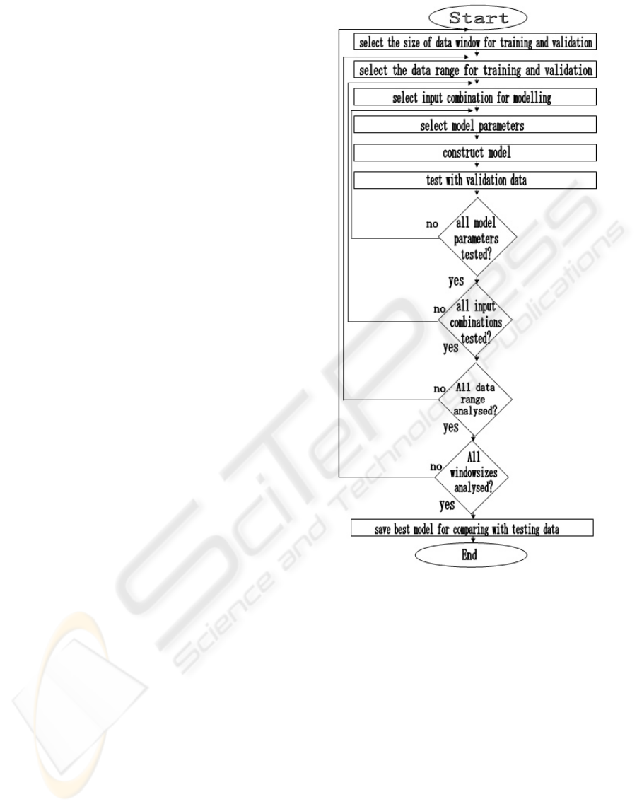
Step 1: Select the size of the time window, M1,

for training and validation. There are two choices:

Start with a small window size and extend it during

the survey, or start with M1=M/2 and decrease it.

Step 2: Select the data range for training and

validation. During the first iteration, choose the

observations m=1…M1 for modelling and

m=M1+1…2M1 for validation. If there are still

observations left, during the next iteration choose

SYSTEMATIC APPROACH TO MODEL-BASED DATA SURVEY

observations m=M1/2+1…1.5M1 for modelling and

m=1.5M1+1…2.5M1 for validation. Use this

overlapping sliding window for all observations.

Step 3: Select the input combination for

modelling. For example, from 15 input variables

using two inputs results in totally 105 combinations,

using 3 inputs 455 and using 4 inputs 1365 different

input combinations. After this, the structure

information of candidate models is stored in tables.

This phase of work is necessary in order to define

inputs that explain most of the output variation. In

the following steps, only inputs proved to be

important are selected for further analysis.

Step 4: Construct the model. All input

combinations are applied one by one in every data

window to model the selected output. At this stage,

only static AR-models are utilised to get

computation less demanding.

Step 5: Test with validation data. If all input

combinations and the whole data range are tested, go

to the next stage. If not, go either to Step 3 or Step 2.

Step 6: Store the best models for testing with

independent data. Best model candidates are stored

in tables, with the root mean square error (RMSE)

and correlation coefficient values of training,

validation and testing data, data range used for

training, variables in models and model degrees (see

for example Table 1). This way it is possible to

reconstruct individual models for further use or

graphical inspection. Model parameters are not

stored in tables, but they can be easily retained on

the basis of table values. All the needed information

for the data survey is then available in result tables.

Step 7: If all window sizes are analysed, the

procedure ends. If not, go to Step 1.

The main stages of the presented data survey

approach are described in Fig. 1.

Figure 1: Flowchart of the data survey approach

Using all the previous phases and input variable

combinations, hundreds of thousands of model

candidates can be constructed and tested. This would

be impossible without the described systematic

procedures.

The data survey method was programmed using

MATLAB® script language and functions in

MATLAB® identification-toolbox. Data survey was

performed with software that makes use of the

collected data sets.

3 RESULTS

Analysis of data from an industrial wood debarking

ICINCO 2005 - SIGNAL PROCESSING, SYSTEMS MODELING AND CONTROL

process was used as a case example to show the

effectiveness of the discussed approach.

3.1 Industrial Wood Debarking

Process

In debarking process, logs are debarked in a drum;

typical dimensions are 5 m of diameter and length of

30 m. Logs scrub each other in the drum and bark is

separated from logs. Bark is removed from the drum

via bark holes in the sides of the drum, logs exit

from the end of the drum for further process stages.

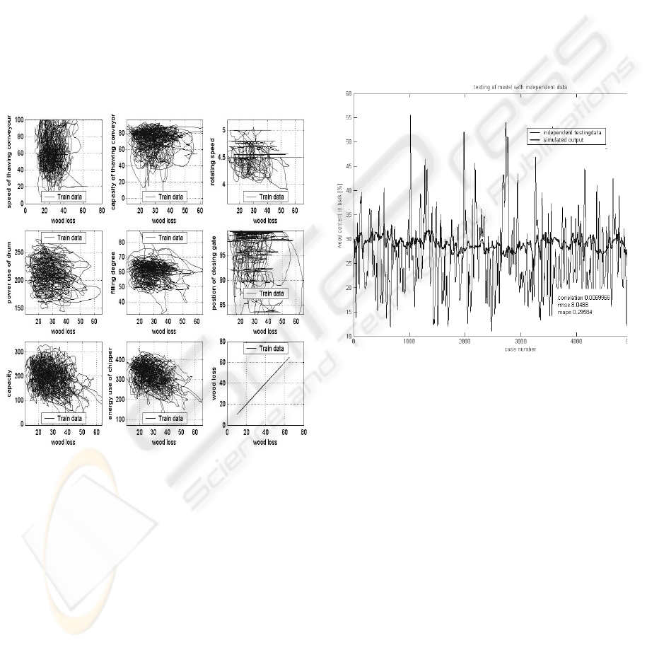
Typical measurements are presented as scatter plots

in Fig. 2 describing the general properties of wood

loss data.

Figure 2: Scatter plot from the measurements of the

debarking drum. Wood loss measurement (output

variable) in x-axis and input variables in y-axis

3.2 Process Identification without

the Data Survey

This section presents a typical example, how linear

model works, if the systematic data survey is not

used.

First, all available measurements of debarking

plant were investigated using cross correlation tables

and graphical presentations. Cross-correlation

analysis was committed for measurements, but all

correlations with wood loss measurement (output)

were only between 0 – ±0.4. Correlation describes

only a linear dependency, so graphical analysis was

the next step.

It was noted that there were no remarkable

dependencies between process measurements and

wood losses (Fig. 2). This was mainly because data

set from a large database incorporated a lot of

different operation conditions. Scatter plot figures

show that modelling wood loss without any

systematic modelling approach will be difficult.

Preliminary identification tests with linear

models showed unsatisfactory results (Fig. 3), when

training data set was selected randomly. In this case,

first 25 % of the data is used for training, next 25%

for validating and the rest 50% for testing.

Figure 3: Comparison of simulated wood losses with

measured data, when training data has been selected

without a prior analysis

3.3 Data Survey with the Model-

based Approach

In this section an example of the data survey is

given. Results were obtained through simulations

with the validation data set.

The procedure described in section 2 provided

the following results: first using four inputs gave

better modelling accuracy for candidates than two or

three. Modelling with five inputs was committed

also later, but the results were not as good as for four

inputs. The parameters used for constructing models

and model goodness values are in Table 1 for some

of best models gained using data survey. The

optimal size of data window for training data

seemed to be quite short, typically from 100 to 400

minutes. Candidate models constructed using the

window sizes of 500-1000 usually failed. From the

SYSTEMATIC APPROACH TO MODEL-BASED DATA SURVEY

result table one can conclude that some segments of

data seemed to be good for training data whereas

some areas contained malfunction data and models

constructed with such data failed. The best model

candidates were selected on the basis of root mean

square error (RMSE), correlation values and visual

appearance of the model behaviour. According to

the result table, the best variables describing wood

losses were (1) rotating speed of the drum, (2) the

filling degree, (3) capacity and (5) the position of

closing gate. This agrees well with the operator

experience from the process.

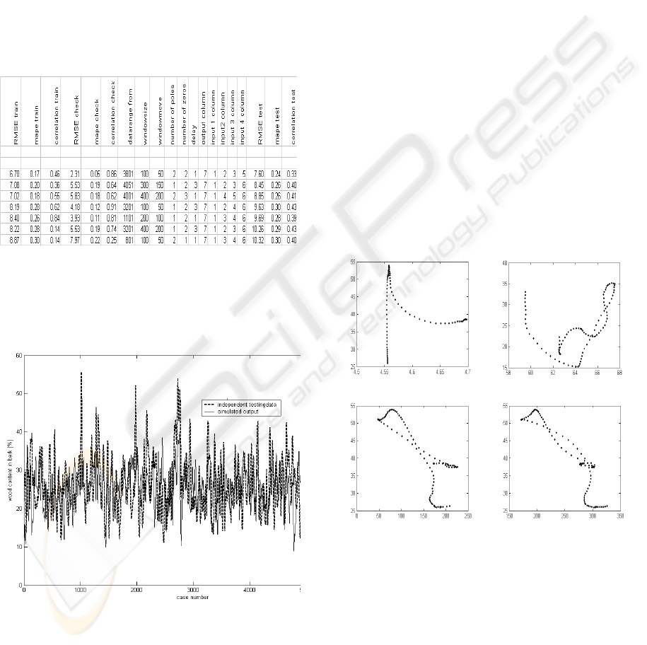
Table 1: Some of the best candidate models gained

utilising data survey

Fig. 4 presents simulation results with

independent testing data, when training data has

been selected automatically (row 1 from Table 1).

Figure 4: Testing wood loss model with independent

testing data, when training data has been selected in the

systematic way

Fig. 5 shows the main process interactions found

after the data survey for four variables that effect to

wood loss of debarking process. For example,

increase in capacity clearly seems to decrease the

wood loss. The relationship between these variables

is similarly recognised by process operators.

4 DISCUSSION

Fig. 2 shows at the first glance that there are no

dependencies between wood loss and input

variables. Modelling with such data will be difficult

as can be seen from Fig. 3, although all the input

combinations were tested. This is because training

data was too large containing too many different

process conditions and changes in the quality of raw

material.

Fig. 5, on the other hand, shows that the data

survey finds the main process interactions. This

suggests that the selection of correct inputs, optimal

data window sizes and optimal data segments

reveals clear interactions between variables. This

may in turn give acceptable results even with very

simple modelling techniques (Fig. 4). Model

development can continue after this with more

sophisticated models.

Rotating speed

Filling degree

Figure 5: Main process interactions according to the data

survey

The optimal size of data windows might vary

with different modelling methods. Another

challenge in this approach is the need for

computation power. Typical calculation times were

from 30 minutes (AR-models) to 12 hours (approx.

100 000 models constructed, validated and tested).

This can be better coped by implementing

calculations in more powerful servers. On the other

RMSE 7.6

MAPE 0.24

Capacity

Chipper power

Wood content in bar

ICINCO 2005 - SIGNAL PROCESSING, SYSTEMS MODELING AND CONTROL

hand, calculation times with the state of art PC are

also reasonable.

Although the presented approach proceeds

systematically, some expertise is useful defining the

correct boundaries for calculating parameters, for

example, data window sizes. If limits are set too

wide, calculation times may increase exponentially.

In this phase, there is not any automated procedure

to select best model candidates from result table and

requires also expertise. This is mainly because the

selection of best model candidates requires also

visual inspection of the model behaviour and is

therefore difficult to automate. In the future, the

approach will be developed more into fully

automated way.

The presented approach can provide successful

results, even if data pre-processing or outlier

removal has failed. This is because data survey can

help to choose data segments containing only

relevant information. Thus, the need for data survey

is evident.

5 CONCLUSIONS

In this paper, a systematic approach for data survey

was presented and applied to wood loss data.

Model candidates using simple dynamic ARX –

models were constructed systematically with

different input combinations, window sizes and data

ranges. The target was to find out the best data sets

for further modelling. Model candidates working

best with validation data were stored and tested with

independent data.

Main process interactions and delays were easily

discovered from structures of the interpretable linear

model candidates. The analysis can thus provide

valuable information also for the model structure

selection. This shows the importance of proper data

survey. It is also one kind of data mining stage: with

the proper data survey, best inputs, correct

interactions between variables and optimal data

window sizes could be found even with linear

modelling methods. Data survey also provides

information about model degrees and delays. This

kind of knowledge discovery is an important step in

process control development.

REFERENCES

Abonyi, J., R. Babuška and B. Feil, 2003. Structure

selection for nonlinear input-output models based on

fuzzy cluster analysis. IEEE International Conference

on Fuzzy Systems, v 1, pp. 464-469

Anctil, F., C. Perrin and V. Andréassian, 2004. Impact of

the length of observed records on the performance of

ANN and conceptual parsimonious rainfall-runoff

forecasting models, Environmental Modelling &

Software, 19, pp. 357-368.

Isokangas A. and K. Leiviskä, 2005. Minimising wood

losses of drum debarking. Accepted to Paper and

Timber magazine.

Kocjančič R. and J. Zupan, 2000. Modelling of the river

flowrate: the influence of the training set selection,

Chemometrics and Intelligent Laboratory Systems, 54,

pp. 21-34.

Linkens, D.A. and M.-Y. Chen, 1999. Input selection and

partition validation for fuzzy modelling using neural

network. Fuzzy Sets and Systems, 107, pp. 299-308.

Ljung, L., 1999. System identification: theory for the use.

Prentice hall, Englewood cliffs, NJ.

Luo, W. and S.A. Billings, 1995. Adaptive model

selection and estimation for nonlinear systems using a

sliding data window, Signal Processing, 46, pp. 179-

202.

Mendes, E.M.A.M and S.A. Billings, 2001. An alternative

solution to the model structure selection problem.

IEEE Transactions on Systems, Man, and Cybernetics

Part A: Systems and Humans, 31, pp. 597-608.

Näsi, J., A. Isokangas and E. Juuso, 2001. Klusterointi

kuorimon puuhäviöiden mallintamisessa. ISBN 951-

42-5894-0.

Prudêncio, R.B.C., Ludermir T.B. and de Carvalho F.A.T.,

2004. A Modal Symbolic Classifier for selecting time

series models, Pattern Recognition Letters, 25, pp.

911-921.

Pyle, D., 1999. Data Preparation for Data Mining.

Morgan Kaufmann, San Francisco, California.

Simon, G., J Schoukens and Y. Rolain, 2000. Automatic

model selection for linear time invariant systems,

Proceedings of the12th IFAC Symposium on System

Identification, SYSID, Santa Barbara, CA, USA, 21-

23 June 2000, Vol. I., pp. 379-384.

Šindelář, R., 2004. Input selection for fuzzy modelling.

Proceedings of the 2nd IFAC Workshop on Advanced

Fuzzy/Neural Control, Oulu, Finland, pp. 13-18.

Sugeno, M. and G. Kang, 1988. Structure identification of

fuzzy model. Fuzzy Sets and Systems, 28, pp. 15-33.

Söderström, T. and P. Stoica, 1988. System identification,

Englewood cliffs, NJ. Prentice Hall.

SYSTEMATIC APPROACH TO MODEL-BASED DATA SURVEY