
OBSTACLE DETECTION BY STEREO VISION,
INTRODUCING THE PQ METHOD
H. J. Andersen, K. Kirk, T. L. Dideriksen, C. Madsen and M. B. Holte
Computer Vision and Media Technology Laboratory
Aalborg University, Denmark
T. Bak
Danish Agricultural Sciences
Denmark
Keywords:
Computer vision, Autonomous mobile robot, Obstacle detection, Stereo vision.
Abstract:
Safe, robust operation of an autonomous vehicle in cross-country environments relies on sensing of the sur-
roundings. Thanks to the reduced cost of vision hardware, and increasing computational power, computer
vision has become an attractive alternative for this task. This paper concentrates on the use of stereo vision for
obstacles detection in cross-country environments where the ground surface can not be modeled as ramps, i.e.
linear patches. Given a 3D reconstruction of the surrounding environment, obstacles are detected using the
concept of compatible points. The concept classify points as obstacles if they fall within the volume of cone
located with its apex at the point being evaluated. The cone may be adjusted adjusted according the physical
parameters of the vehicle. The paper introduces a novel Projection and Quantification method that based on
vehicle orientation rotates the 3D information onto an intuitive two dimensional surface plot and quantifies the
information into bins adjusted to the specific application. In this way the search space for compatible points
is significantly reduced. The new method is evaluated for a specific robotic application and the results are
compared to previous results on a number of typical scenarios. Combined with an intuitive representation of
obstacles in a two dimensional surface plot, the results indicate a significant reduction in the computational
complexity for relevant scenarios.
1 INTRODUCTION
Robotics, control, and sensing technology are today
at a level, where it becomes interesting to investi-
gate the development of mobile autonomous vehicles
to off-road equipment domains, such as agriculture
(Stentz et al., 2002; Bak and Jakobsen, 2004), lawn
and turf grass (Roth and Batavia, 2002), and construc-
tion (Kochan, 2000). Efficient deployment of such ve-
hicles would allow simple, yet boring, tasks to be au-
tomated, replacing conventional machines with novel
systems which rely on the perception and intelligence
of machines.
One of the most challenging aspects of cross-
country autonomous operation is perception such as
in agricultural fields, small dirt roads and terrain cov-
ered by vegetation. In cases localization may be
achieved using technology such as GPS, and paths
planned a priori or according to specific application
structures, the ability to perceive, or sense, the sur-
rounding environment is essential to driving and thus
to the deployment of autonomous vehicles. The per-
ception can be performed by radio, acoustic, mag-
netic, and tactile sensors. These active sensors or a
combination thereof can measure obstacles (Langer
et al., 1999; Borenstein and Koren, 1998); however,
thanks to the reduced cost of image acquisition de-
vices and to the increasing computational power of
computer systems, computer vision has recently be-
come a popular method for sensing the surround-
ing environment. In comparison with active sensors,
computer vision does not interfere when several vehi-
cles are moving simultaneously in the same environ-
ment, thereby providing more flexibility and a less ex-
pensive solution. On the other hand, computer vision
is a computationally complex process, and there are
problems intrinsic to the outdoor environment, such
as lighting and dynamic range effects, which causes
false positives and false negatives.
Here the focus is on obstacle detection using three-
dimensional information from a binocular stereo vi-
sion system. Stereo images are acquired simultane-
ously from different points of view, and we search
for objects which can obstruct the path of a vehicle.
The problem is reduced to identifying the free space
(the area into which the vehicle can move safely).
250
J. Andersen H., Kirk K., L. Dideriksen T., Madsen C., B. Holte M. and Bak T. (2005).
OBSTACLE DETECTION BY STEREO VISION, INTRODUCING THE PQ METHOD.
In Proceedings of the Second International Conference on Informatics in Control, Automation and Robotics - Robotics and Automation, pages 250-257
DOI: 10.5220/0001168602500257
Copyright
c
SciTePress

The development of the obstacle detection algorithm
has been guided by application to the agricultural ap-
plication domain. While the environment in devel-
oped agriculture is semi-structured and well main-
tained, there may be regions (obstacles), which vehi-
cles should not move into. Obstacles depend on vehi-
cle capabilities and include humans, trees, big rocks,
ditches, and other depressions (potentially filled with
water). As result it is not feasible to rely on horopter
based methods (Badal et al., 1994; Se and Brady,
1998).
This paper first outlines the background in terms
of stereo vision and introduces obstacle detection us-
ing the concept of compatible points. Next, a novel
projection and quantification method is introduced
which projects the 3D reconstructed point cloud onto
a global ground plane and quantifies the projected the
points into bins. In Section 3, the novel method is
evaluated by a comparative study with the recently
introduced obstacle detection in (Manduchi et al.,
2005). The complexities of the algorithms are com-
pared and noise suppression discussed. Finally, the
results are discussed and conclusions given.
2 MATERIAL AND METHOD
2.1 Stereo Vision
Three-dimensional information may be acquired in
many different ways. However, in this study we will
concentrate on the use of binocular stereo, i.e., two
cameras giving a right and a left image. In the follow-
ing, it will be assumed that the cameras used are inter-
nally and externally calibrated. Internal camera para-
meters include focal length, center pixel position, and
geometric distortion. External parameters describe
the positions and orientations of the cameras.
The key to success in stereo vision is to find match-
ing elements in our stereo pair of images. The el-
ements may be lines, edges, etc., in feature-based
matching, or pixels as in area based-matching. The
problem is to find the element in the right image
which has the highest similarity to an element in the
left image.
The search space for matching image elements is
limited considerably by the epipolar constraint. This
constraint exploits that, given a point in one image,
the corresponding point in the second image will al-
ways lie on a line, called the epipolar line. Assuming
a pinhole camera model, the epipolar line is the pro-
jection on the second image plane of the line spanned
by the image point and the focal point of the first cam-
era (Trucco and Verri, 1998).
The epipolar constraint reduces the correspondence
search space from two dimensions (the whole image)
to one dimension (a single line). However, the search
may be eased further by rectifying the stereo images
before the search. Rectification consists of transform-
ing the images to appear as if they were obtained with
parallel cameras with equal focal lengths (Fusiello
et al., 1997). After rectification, the epipolar lines
become horizontal, so that all corresponding pairs of
image elements lie on the same image rows.
From the two rectified images the disparity d may
be calculated as the horizontal displacement between
the reference pixel in the left image and the candidate
pixel in the right image, that is, x
r
= x
l
+ d. (Fig. 1).
Due to the geometry of parallel axes, decreases with
increasing depth.
From the disparity map, the 3-dimensional recon-
struction of the scene may be determined by triangu-
lation. Ideally, the two rays from the left and right
images should cross a in point. However, due to
the quantification in the imaging process this is sel-
dom the case. Hence, the method of triangulation
with non-intersecting rays (Trucco and Verri, 1998)
is used for the reconstruction.
2.2 Compatible Points and Obstacle
Detection
Below, the concept of compatible points, as intro-
duced by (Manduchi et al., 2005), will be presented.
The concept addresses the problem that in cross-
country environments the ground surface can seldom
be modelled as ramps, i.e linear patches. Obstacles
in terms of two distinct points in space are defined as
follows:
Definition 1
Two 3D points p
1
and p
2
are called compatible with
one another if the following two condition are met:
1. Their difference in height is larger than H
min
but
smaller than H
max
.
H
min
< |p
2,y
− p
1,y
| <H
max
2. The lines joining them form an angle with the
horizontal plane larger than θ
max
.
|p
2,y
− p
1,y
|
p
2
− p
1
> sin θ
max
Definition 2
Two 3D points, p
1
and p
2
, are defined as belonging
to the same obstacle if one of the following two
conditions are met:
1. The 3D points, p
1
and p
2
, are compatible.
2. A chain of compatible point pairs linking p
1
and
p
2
exists.
OBSTACLE DETECTION BY STEREO VISION, INTRODUCING THE PQ METHOD
251
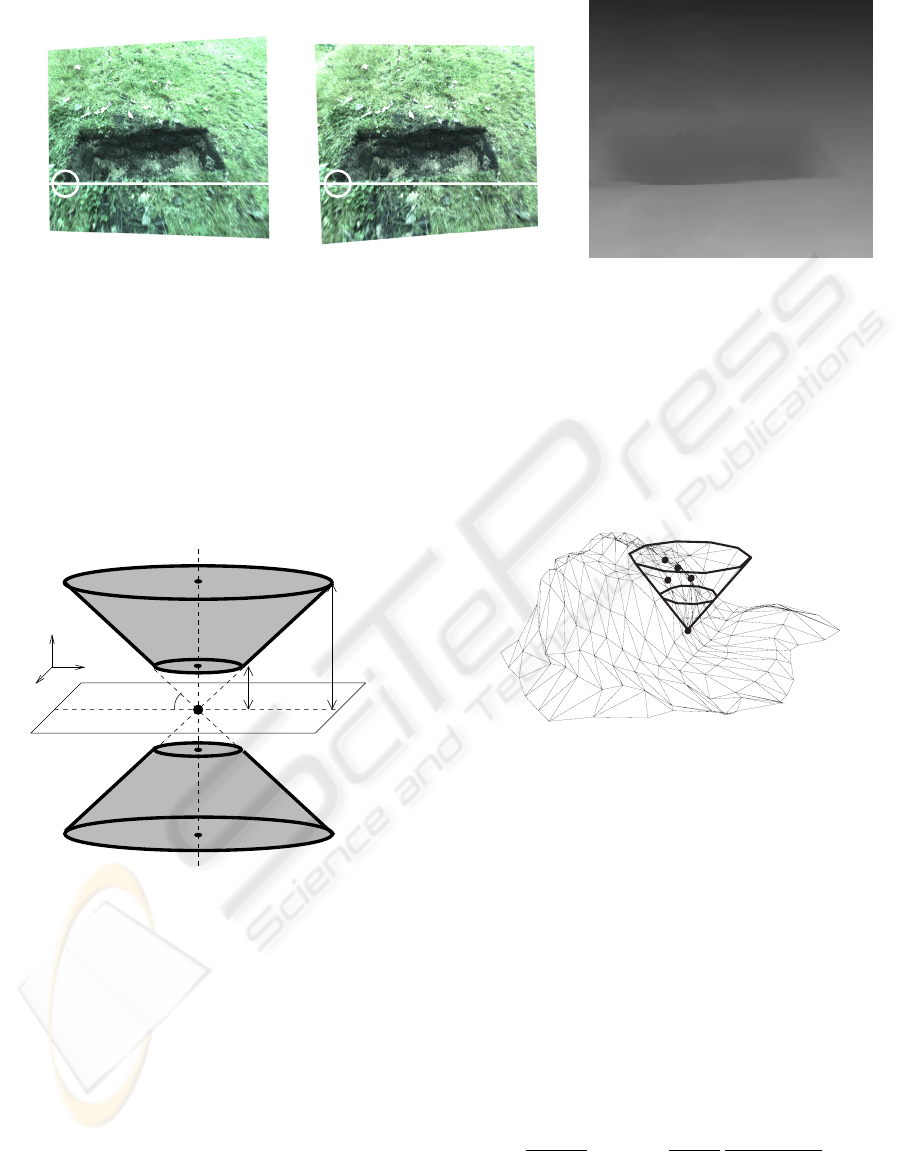
(a) Left rectified image. (b) Right rectified image. (c) The disparity map.
Figure 1: Calculation of disparity for a hole in a grass lawn, i.e. a concave obstacle. The white lines indicates the epipolar
lines in the two images. The objective is to find the pixel in the right image with the highest similarity to the pixel in left
image, illustrated with white circles. The disparity is the displacement between the two pixels.
The two definitions translate, for a given point p,
into a volume of two symmetrical truncated cones in
3D space, with apexes placed in p. Points located
inside the volume are compatible with the given point
p, figure 2.
P
H
min
H
ma
x
θ
max
Figure 2: Geometric interpretation of the parameters H
min
,
H
max
and θ
max
.
According to definition 1 and 2, the size and shape
of the cone volume depends on the variables H
min
,
H
max
and θ
max
. These parameters may all be re-
lated to the physical dimension of a specific vehicle.
H
max
states the height at which it is able to drive un-
der and/or the distance at which it can pass between
two obstacles. H
min
defines the height of undulations
in the surface which the vehicle can easily pass, and
θ
max
the slope rate it is able to climb.
Manduchi et al. 2005 suggested two methods for
detection of obstacles based on the compatible point
concept, respectively, OD1 and OD2. In OD1, both
the upper and lower cone at a given point are consid-
ered whereas for the OD2 method only the upper cone
is considered for classification of points. The two ap-
proaches reach the same result and in the following
only OD2 will be used. Figure 3 illustrates the princi-
ple in a synthetic scene with four compatible points.
Figure 3: Classifications of obstacle points by the compati-
ble points method (vertex are the reconstructed points). The
cone apex is placed in the point being evaluated. The four
points which falls inside the cone together with the point
being evaluated are all classified as obstacle points.
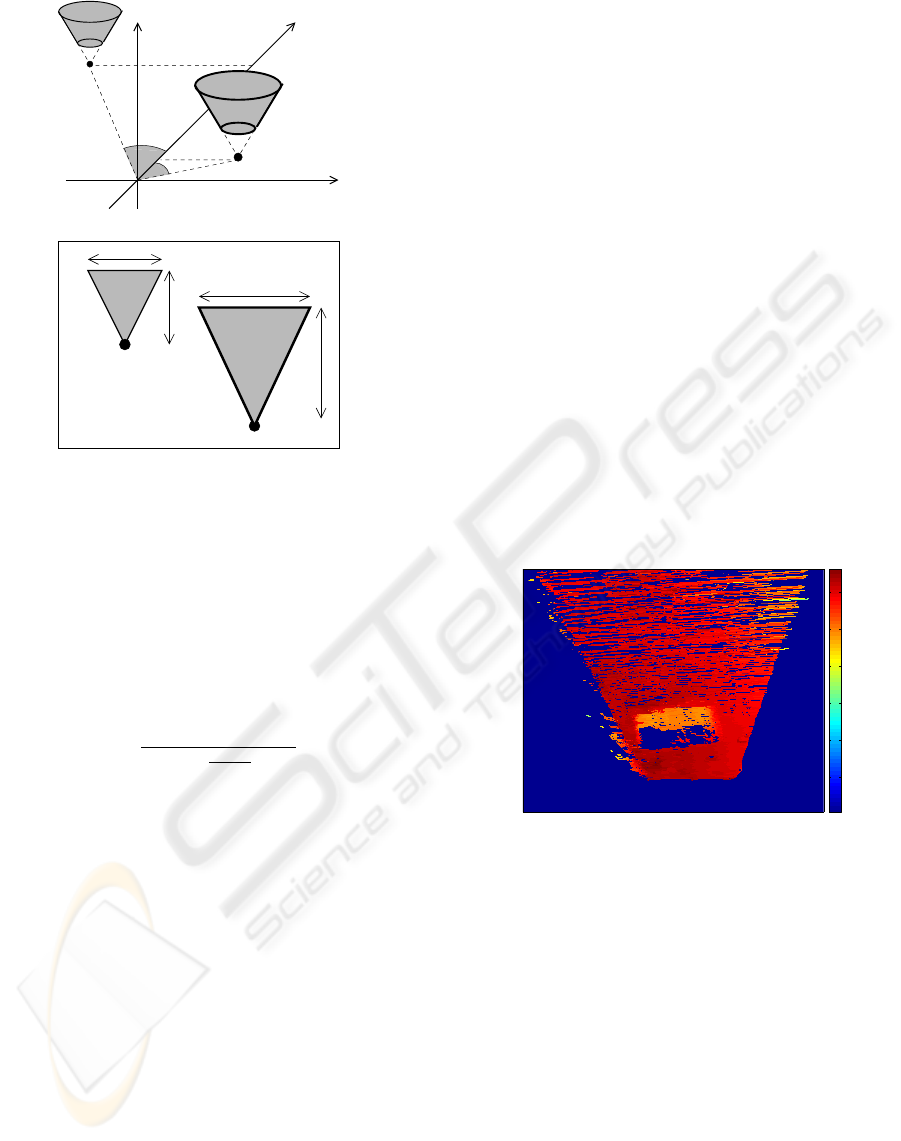
A computational yet expensive part of the algo-
rithm is the search for 3D points located inside the
truncated cone. A naive implementation would be to
search through all 3D points, evaluating each one. To
reduce the search space Manduchi et. al propose a
method for limitation of the search space by projec-
tion of the truncated cones onto the disparity map, as
illustrated in figure 4. For projection, the width and
height of the triangles b and h as illustrated in figure
4, are determined by:.
h =
H
max
f
p
z
b =2
H
max
f
p
z
1
tan θ
max
cos v
(1)
Where f is the focal length of the camera, p
z
is the
z coordinate of the point and v is the azimuth angle.
As a result, the search may be limited to 3D points
ICINCO 2005 - ROBOTICS AND AUTOMATION
252
P
1
P
2
v
v
2
1
y
x
z
Disparity map
b
P
1
P
2
b
h
h
Figure 4: Reducing the 3D search space by projection of
the cones onto the disparity map. Top truncated cones in
3D. Bottom their projection onto the disparity map
included in the projected truncated cones in the dis-
parity map. However, eq. 1 is only valid in the ideal
case, where the vehicle does not pitch or roll. In order
to compensate for this Manduchi et. al. introduced a
pitch compensation factor, α, by:
α =
1
cos γ ±
H
max
p
z
sin γ
(2)
Where γ is the immediate pitch angle. The result-
ing triangle is adjusted by multiplication of h with α,
Vehicle roll is simply compensated by an expansion
of the triangle by addition of a factor to both b and h.
2.3 Introducing the PQ method
Below, the new method Projection and Quantifica-
tion, PQ for representation of the three-dimensional
point cloud from the reconstructed scene will be in-
troduced. The method operates on the counter ro-
tated point cloud (P
cr
) according to the robots pitch
(R
pitch
) and roll (R
roll
) and the default orientation of
the stereo setup (R
default
), by:
P
cr
=(R
pitch
R
roll
R
defualt
)P (3)
where P is a matrix 3 × m gathering all the recon-
structed points (m = number of points), and R
∗
rota-
tion matrices. After the counter rotation, the method
consists of the following two steps:
P - step which Project the counter rotated 3D point
cloud onto the XZ-plane, (i.e. the global ground
plane)
Q - step which Quantify the projected point cloud
into predefined bins on the XZ-plane
The counter rotated and quantified point cloud may
be regarding as a two dimensional surface plot. This
will be denoted as the PQ-representation. A bin may
contain several points. Further, the quantification may
be adjusted to the specific application i.e. the size of
the robot and/or size of the obstacles. A fine quan-
tification will make it possible to detect small obsta-
cles whereas a coarser one will increase the opera-
tional speed. For representation of the points quanti-
fied into a specific bin, several metrics may be used
as: the mean, max, min, median etc. In this study,
the median value of the points quantified into a given
bin will be used as a representation of its estimated
height. The median value is chosen due to its capa-
bilities of suppressing salt and pepper noise, which is
likely to occur in 3-dimensional reconstructions. The
PQ-representation of the images in figure 1, is shown
in figure 5.
X
Z
−180
−160
−140
−120
−100
−80
Figure 5: The PQ representation of the images in figure
1.The bins are represented by their median values in cm
as the distance from the camera setup. Dark blue bins are
empty. The hole in the lawn is app. 120 cm broad, 30 cm
wide and 25 cm deep. The bin size is 1 cm x 1 cm at ground
surface. The color bar indicates distance from the cameras,
n.b. dark blue areas is occluded or not within the field of
view.
As the point cloud is counter rotated the projection
of the truncated cones onto the PQ-representation is
straight forward. In the counter rotated point cloud
the center axis of the cone becomes perpendicular to
the XZ-plane and hence it may be discretized accord-
ing to the quantification of the PQ-representation, as
illustrated in figure 6.
As a result, detection of compatible points may be
done simply by evaluating whether the median value
OBSTACLE DETECTION BY STEREO VISION, INTRODUCING THE PQ METHOD
253
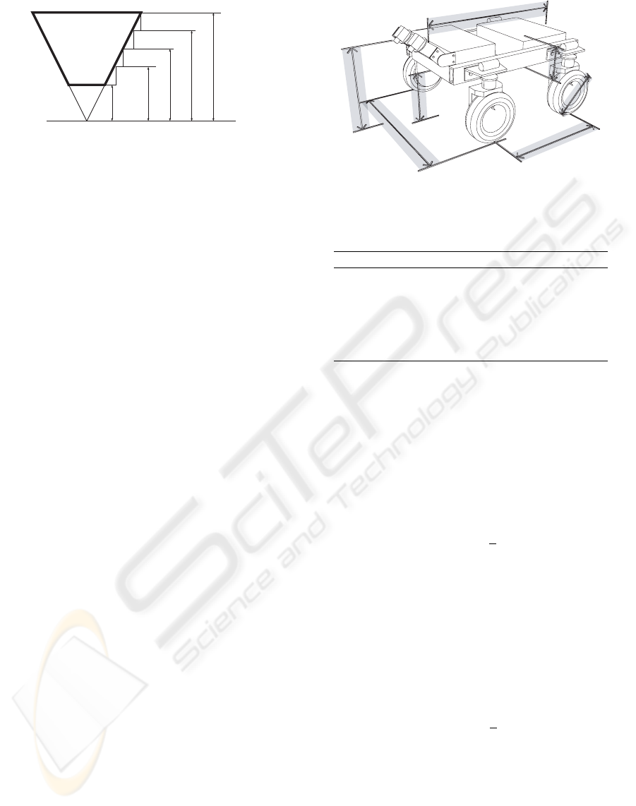
H
min
H
max
H
1
H
2
H
3
Ground Surface
Figure 6: Side view of the discretized truncated cone. H
min
indicates the minimum value of a bin before it is classified
as an obstacle point. H
1
,H
2
, and H
3
is the lower limit val-
ues for when a point is not classified as an obstacle, i.e. the
value increases as we move away from the apex according
θ
max
. All bins with a value bigger than H
max
is not classi-
fied as obstacles.
of a bin is bigger than the lower limited of the discrete
truncated cone, i.e. greater than H
min
,H
1
,H
2
,H
3
in
figure 6, and lower that the maximum limit H
max
, i.e
the top of the cone.
3 COMPARING THE PQ AND
OD2 METHODS
The following section will present a comparative
study of the PQ and OD2 methods. The unbound
complexity of the two methods will be evaluated.
However, when working with computer vision meth-
ods the unbound complexity is not that interesting
from a practical point of view, as the image dimen-
sions give a very concrete bound for complexity of
the methods. Hence a more concrete comparison will
be investigated according to a specific robot.
3.1 Robot setup
For the comparison of the two methods the au-
tonomous platform (Bak and Jakobsen, 2004), will be
used (figure 7). From the physical dimensions of the
robot the setting of the parameters for the OD2 and
PQ methods may be determined. Table 1 summarizes
the values used in the following simulations and ex-
perimental work.
The cameras in the stereo setup were mounted at a
height of 75 cm and had a base-line of 16.4 cm, which
gave an uncertainty in depth of 1.84 cm at a distance
of 1.06 m along the optical axis. The image field of
view covered an area from the front wheels to app.
150 cm in front of the robot and was app. 140 cm
wide in the center of the image field.
75 cm
100 cm
100 cm
46 cm
60 cm
27 cm
150 cm
Figure 7: The physical dimensions of the API robot.
Table 1: Parameters used in the comparative study.
Parameter Value
H
min
10 cm
H
max
121 cm
θ
max
60
◦
Camera tilt angle 45
◦
Image resolution 1280 × 1024
PQ quantization 1 cm × 1cm
3.2 Worst case Complexity
For the OD2 method, a triangle is imposed in the dis-
parity image for all pixels. Further, depending on the
resolution of the disparity map, a fraction a of the im-
age pixels shall be compared with the pixels inside the
projected triangle. This gives a worst case complexity
of O(n
2
):
n(c + n
1
a
) (4)
where c denotes the constant for projection of the tri-
angles and a the fraction of pixels inside the projected
truncated cone.
For the PQ method, all 3D reconstructed points are
first counter rotated and projected onto the XZ-plane.
After this operation, a fraction of the bins depending
on the quantification of the XZ-plane must be com-
pared with one another. This also gives a worst case
complexity of O(n
2
):
n(d + n
1
b
) (5)
where d denotes the constant for the counter rotation
and projection of the 3D reconstructed points and b
the fraction of bins which has to be compared.
3.3 Bounded Complexity
For illustration of the two methods, operational char-
acteristics three different scenarios are simulated (fig-
ure 8). A flat surface (plan lawn), a vertical obstacle
ICINCO 2005 - ROBOTICS AND AUTOMATION
254
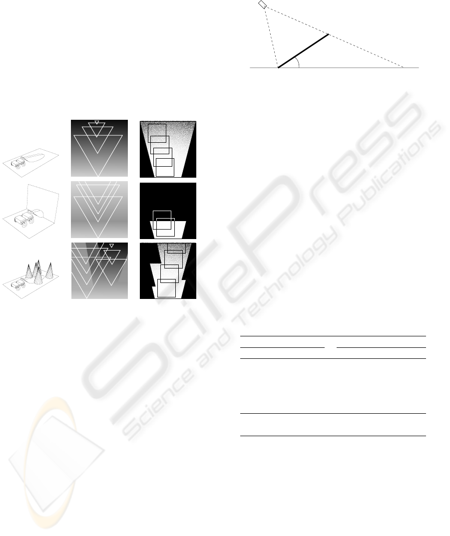
(a wall), and a landscape with cone obstacles (trees).
The simulations clearly illustrate the main difference
between the two methods. For the OD2 method, the
whole disparity has to be searched in all three simula-
tions, whereas for the PQ method the search space is
limited to include only the bins with points projected
into them. This gives a severe reduction in the search
space for the vertical obstacle, where the area in black
may be excluded. Also, the size of the squares are un-
affected by the location in the PQ-representation com-
pared to the imposed triangles for the OD2 that in the
worst case almost span the whole disparity map, i.e
figure 8.
Figure 8: Illustration of the search space reduction for the
OD2 and PQ methods for the API robot. 1st column, illus-
tration of different scenarios. Top row, flat surface scenario.
Middle row, vertical obstacle. Bottom row, cone obstacles.
2nd column, the disparity map with triangles imposed illus-
trating the span from the largest to the smallest search space
reduction. 3rd column, the PQ-representation with squares
illustrating the reduction of the search space.
For a more quantitative comparison of the bounded
complexity the, two methods were evaluated by sim-
ulating the rotation of a planar surface in front of the
robot (figure 9). The angle by V was varied from from
0 to 90 degrees in steps of 5 degrees. At each step
the number of comparison for the two methods was
logged.
The result of the simulation is plotted in figure 11.
The figure clearly illustrates the characteristics of the
two methods. The PQ method has its worst perfor-
mance at an angle of 0 degree with increasing num-
ber of comparisons until 90 degrees. For the OD2
method, the characteristics are just the opposite. This
method has the lowest number of comparisons at 90
degrees with increasing number of comparisons till
0 degrees is reached. However, at all angles the PQ
method is significantly better than the OD2 method,
ranging from a factor of 44 at 0 degrees and 270 at 90
degrees.
V
Figure 9: The ground surface used in the simulated compar-
ison.
3.3.1 Noise suppression
In order to evaluate the PQ noise suppression, the ro-
bot traveled across a flat gras lawn. For estimation
of the disparity map the method in (Birchfield and
Tomasi, 1999), was used. Five pairs of stereo images
were captured. In all cases the undulations in the sur-
face were not exceeding that of H
min
threshold of 10
cm, so pixels classified as obstacles may have been
regarded as being due to faults in the disparity esti-
mation. An example of the scenario is illustrated in
figure 10.
Table 2: Noise suppression. Points denotes the number of
data points addressed and %-Faults the percentage of points
incorrect classified as obstacles. For the OD2 method this
correspond to all image pixels, i.e. 1280 × 1024 equals
687219, whereas for the PQ method there is a reduction in
the points to process due to the quantification.
PQ OD2
Points %-Faults Points %-Faults
48014 2.6 687219 11.9
47514 3.5 687219 13.0
46478 4.3 687219 12.2
45260 7.0 687219 24.7
45157 17.5 687219 37.3
In average:
46485 6.9 687219 19.8
Table 2 summarize the result of the noise suppres-
sion evaluation. First, as with the bounded complex-
ity, the impact of the quantification in the PQ method
reduces in average the necessary points to process by
a factor 15. Further, the median representation of the
bin values reduces the percentage of incorrect classi-
fied points by approximately a factor 3.
4 DISCUSSION
A new method for representation of the reconstructed
3D points cloud from a binocular stereo vision sys-
OBSTACLE DETECTION BY STEREO VISION, INTRODUCING THE PQ METHOD
255
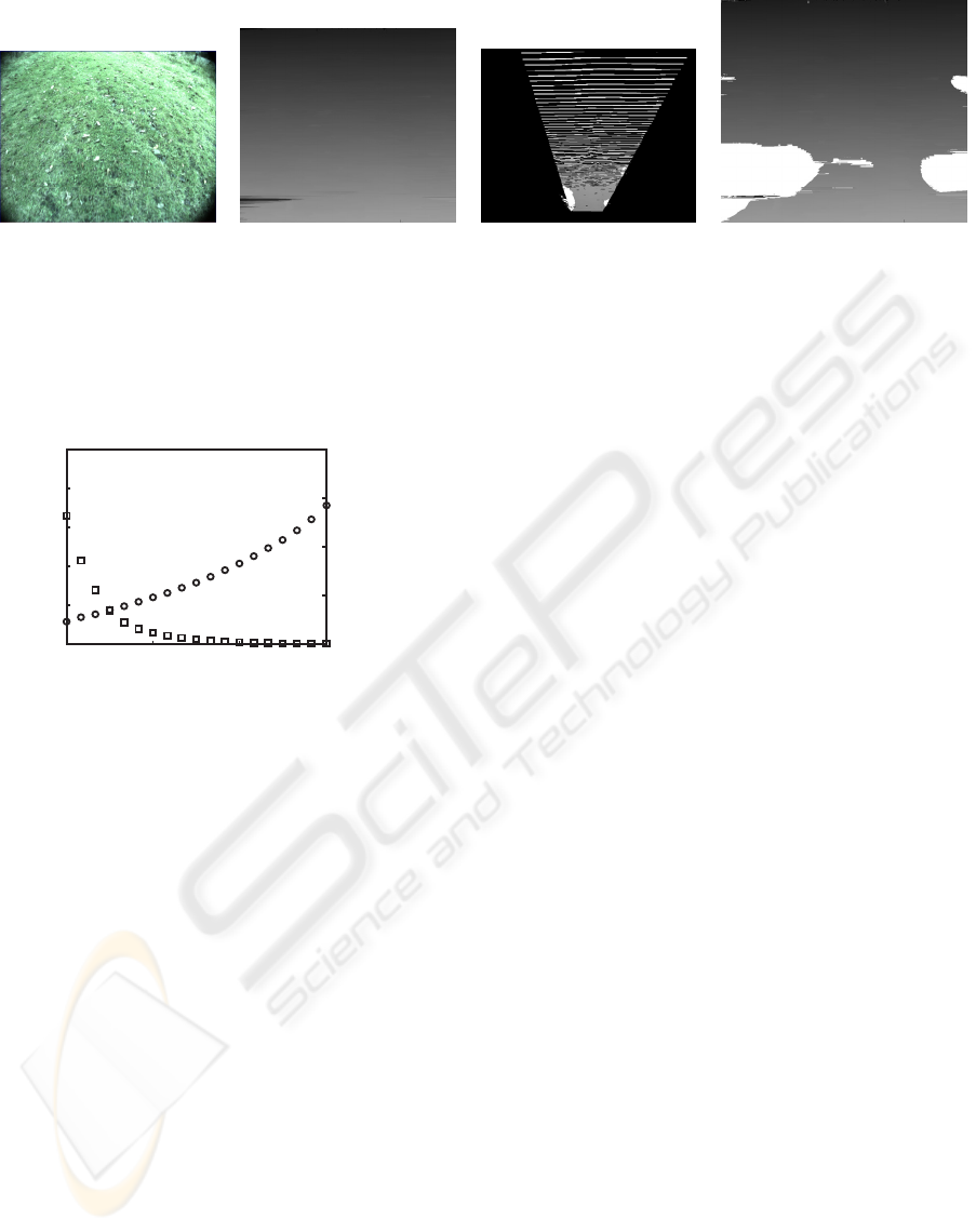
abc d
Figure 10: Noise suppression capabilities of the PQ and OD 2 methods. a) Left image of a flat grass lawn. b) Disparity
map. c) PQ representation, white areas are incorrectly classified as obstacles. d) Results of the OD2 method white areas are
incorrectly classified as obstacles.
00
0
2
4
6
8
10
x10
11
0
30
60
90
0
1
2
4
3
x10
9
Number of Comparisons
Degrees
The OD2 method
The PQ method
Figure 11: Number of comparison for OD2 and PQ methods
when a flat ground surface is rotated in front of the robot, as
illustrated in figure 9. The OD2 method is illustrated with
a circle and the PQ with a square. Notice the difference in
the magnitude of the two y-axis.
tem is presented. For evaluation of the method it is
compared to the recently introduced OD2 method by
(Manduchi et al., 2005). In the evaluation problems
regarding occluded areas has not been addressed.
However, in terms of computational demand occluded
areas will have the same impact on the two methods.
The question is more how these shall be classified. A
conservative approach is to regard all occluded areas
as obstacles areas, i.e. the robot shall not move into
these.
The comparative study has in this study been based
a specific robotic platform. Whether this platform fa-
vor one of the method is not evaluated. However the
physical dimension of the robot and the mounting of
the stereo setup may be regraded as being very realis-
tic for a cross-country operating robot.
More critical is the evaluation of the noise sup-
pression. This study is more an evaluation of what
may be called the implicit noise suppression of the
PQ-method. Clearly, the performance of the OD2-
method may be improved by median or other filter-
ing techniques of the disparity map. However, these
method will also increase the performance of the PQ-
method. Hence these results shall only been seen as
an example of the implicit noise suppression due to
the median representation of the bin values in the PQ-
representation.
5 CONCLUSION
This paper addressed the problem of identifying ob-
stacles for an autonomous vehicle operating in a
cross-country domain. A novel algorithm was pre-
sented based on previous results from (Manduchi
et al., 2005). The new Projection and Quantifica-
tion method projects the 3D information from a stereo
vision system into the surface plane in front of the
robot and quantifies the depth information into bins
that may be adjusted to the specific application. The
bins allow quantification of a cone representing ter-
rain that should not be traversed by the vehicle and
represents both positive and negative obstacles typi-
cally encountered in cross-country environments. The
new algorithm simplifies the computation compared
to (Manduchi et al., 2005) for a number of specific
scenarios. The result is a modified algorithm (the PQ
method), that provides an intuitive representation of
the surrounding environment and simple detection of
obstacles.
REFERENCES
Badal, S., S. Ravela, S., Draper, B., and Hanson, A. (1994).
A practical obstacle detection and avoidance system.
In 2nd IEEE Workshop on Applications of Computer
Vision, pages 97–104.
Bak, T. and Jakobsen, H. (2004). Agricultural robotic plat-
ICINCO 2005 - ROBOTICS AND AUTOMATION
256

form with four wheel steering for weed detection.
Biosystems Engineering, 87(2):125–136.
Birchfield, S. and Tomasi, C. (1999). Depth discontinu-
ities by pixel-to-pixel stereo. International Journal of
Computer Vision, 35(3):269–293.
Borenstein, J. and Koren, Y. (1998). Obstacle avoidance
with ultrasonic sensors. IEEE Journal of Robotics and
Automation, 4(2):213–218.
Fusiello, A., Trucco, E., and Verri, A. (1997). Rectification
with unconstrained stereo geometry. In Proceeding
of the British Machine Vision Conference, pages 400–
409.
Kochan, A. (2000). Robots for automating construction
- an abundance of research. The Industrial Robot,
27(2):111–113.
Langer, D., Mettenleiter, M., Hartl, F., and Frohlich, C.
(1999). Imaging laser radar for 3-d surveying and cad
modelling of real world environments. In Proceedings
of the International Conference on Field and Service
Robotics, pages 13–18.
Manduchi, R., Castano, A., Talukder, A., and Matthies, L.
(2005). Obstacle detection and terrain classification
for autonomous off-road navigation. Autonomous Ro-
bots, 18:81–102.
Roth, S. A. and Batavia, P. (2002). Evaluating path tracker
performance for outdoor mobile robots. In Automa-
tion Technology for Off-Road Equipment.
Se, S. and Brady, M. (1998). Stereo vision-based obsta-
cle detection for partially sighted people. In Proceed-
ings of Third Asian Conference on Computer Vision
ACCV’98, pages 152–159.
Stentz, A. T., Dima, C., Wellington, C., Herman, H., and
Stager, D. (2002). A system for semi-autonomous
tractor operations. Autonomous Robots, 13(1):87–
103.
Trucco, E. and Verri, A. (1998). Introductory Techniques
for 3-D Computer Vision. Prentice Hall.
OBSTACLE DETECTION BY STEREO VISION, INTRODUCING THE PQ METHOD
257
