
A NEW APPROACH TO AVOID OBSTACLES IN MOBILE ROBOT
NAVIGATION: TANGENTIAL ESCAPE
Andre Ferreira, Mario Sarcinelli Filho and Teodiano Freire Bastos Filho
Department of Electrical Engineering
Federal University of Espirito Santo
Av. Fernando Ferrari, 514
29075-910 Vitoria-ES, BRAZIL
Keywords:
Mobile robots, Robot control, Obstacle avoidance, Impedance-based control, Tangential escape.
Abstract:
This paper proposes a new strategy for obstacle deviation when a mobile robot is navigating in a semi-
structured environment. The proposed control architecture is based on a reactive approach, thus demanding
low computational effort. It allows the robot to navigate from a starting point to a destination point without
colliding to any obstacle in its path. The deviation from an obstacle is performed according to an escape angle
calculated so that the new robot orientation is tangent to the obstacle. It is shown that such strategy generates
more efficient trajectories, in the sense that the destination point is reached in less time while saving energy and
reducing the demand on the robot motors. Another meaningful feature of the proposed strategy is that it also
allows to implement the behaviors Wall Following and Corridor Following with no additional computation.
1 INTRODUCTION
When a mobile robot is navigating in an unstruc-
tured environment it is very important to assure that
it will not collide to any obstacle. Several meth-
ods, like Edge Detection (Kuc and Barshan, 1989),
Certainty Grid (Elfes, 1987), Potential Field (Khatib,
1986), Virtual Force Field (VFF) (Borenstein and Ko-
ren, 1989), Vector Field Histogram (VFH) (Boren-
stein and Koren, 1991) and Nearness Diagram (ND)
(Minguez and Montano, 2004), have been used to
avoid obstacles in mobile robot navigation. Some of
them are tailored for reactive navigation and others
are more suitable to deliberative navigation, where a
map of the robot working environment is built (Fox
et al., 1997; Brock and Khatib, 1999; Althaus and
Christensen, 2002).
The VFH, VFF and Certainty Grid methods are tai-
lored for deliberative navigation. They use data com-
ing from the robot sensors to build a detailed map of
the environment, which is used to plan the trajectory
the vehicle should follow. Such methods generally
require a lot of computation and loose effectiveness
upon any change in the robot working environment.
Regarding reactive navigation, the robot has no a
priori knowledge about the environment surrounding
it, except, perhaps, that it is a plain indoor environ-
ment. Then, to plan a trajectory is not possible, since
a map of the environment is not available. The idea is
that perceptions are tightly related to actions, result-
ing in simplicity and low computational effort. Envi-
ronmental changes are not a problem as well, when
reactive navigation is adopted. Therefore, reactive
navigation is more suitable to semi-structured envi-
ronments, while deliberative navigation is more suit-
able to structured environments. The Edge Detection
and the Potential Field methods, among those previ-
ously mentioned, are methods compatible to reactive
navigation.
This paper recalls obstacle avoidance in mobile ro-
bot navigation, and proposes a new approach to this
topic, as it will be detailed in the sequence. For be-
ing extensively used as a reactive control architecture,
the Impedance Based Control (Hogan, 1985; Secchi
et al., 2001), which uses the concept of Artificial Po-
tential Field, is adopted as the starting point. Thus,
Section 2 describes this obstacle avoidance method
and presents a simulated example using it. In the se-
quence, Section 3 describes a modification here pro-
posed to the impedance based control and presents a
simulated example using the new strategy for avoid-
ing obstacles. Next, Section 4 presents two experi-
ments using the new strategy here proposed to avoid
obstacles. Finally, Section 5 highlights the main con-
clusions.
The simulations presented in Section 2 and Sec-
341
Ferreira A., Sarcinelli Filho M. and Freire Bastos Filho T. (2005).
A NEW APPROACH TO AVOID OBSTACLES IN MOBILE ROBOT NAVIGATION: TANGENTIAL ESCAPE.
In Proceedings of the Second Inter national Conference on Informatics in Control, Automation and Robotics - Robotics and Automation, pages 341-346
DOI: 10.5220/0001169403410346
Copyright
c
SciTePress
tion 3 were accomplished using the simulator that
accompanies the Pioneer 2-DX mobile robot, while
the experimental results were obtained using the Pio-
neer 2-DX itself, with an onboard computer based in
the Intel Pentium MMX 266 MHz processor having
128 MBytes of RAM and running the Linux operating
system. The sensors used are 16 ultrasonic sensors in
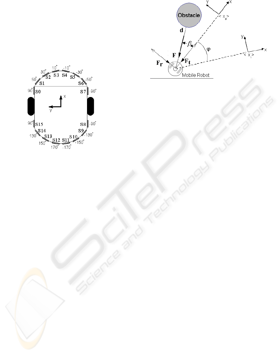
a ring distributed like depicted in Fig. 1.
Figure 1: Sonar distribution for the Pioneer 2-DX platform.
2 THE IMPEDANCE-BASED
CONTROL SYSTEM
This control system uses the concept of generalized
or extended impedance to represent the relationship
between the robot movement and a fictitious repul-
sive force (Hogan, 1985; Secchi et al., 2001). Such
a repulsive force is a function of the distance robot-
obstacle. A contact robot-obstacle should be avoided,
what is accomplished by generating a repulsive force
that increases when the robot gets closer to the obsta-
cle.
2.1 Describing the Impedance Based
Control System
Fig. 2 shows a situation in which an obstacle is de-
tected by the robot sensors. The repulsive force F is
generated, causing a temporary displacement of the
goal point x
d
, which allows the robot to avoid the ob-
stacle by changing its heading angle. The components
of the force F — F
t
(the component coinciding with
the robot orientation) and F
r
(the component normal
to the robot orientation) — are also represented.
The magnitude of the repulsive force F the obsta-
cle exerts on the robot is calculated as (Secchi et al.,
2001)
F = a − b[d − d
min
]
2
, (1)
Figure 2: The fictitious force generated by an obstacle.
where a and b are positive constants related by a =
b[d
max
− d
min
]
2
, d
min
is the minimum distance the
sensors are able to measure, d
max
is the maximum
distance intended to cause a nonzero fictitious repul-
sive force and d is the smallest robot-obstacle distance
currently measured by the robot sensors. Notice that
d
min
< d < d
max
, and d
max
characterizes the re-
pulsion zone, defined as the region inside which the
fictitious repulsive force has a non-zero value.
An impedance Z(s) is then defined as
Z(s) = Bs + K, (2)
where B and K are positive constants representing
the damping and spring effect of the interaction robot-
obstacle in the repulsion zone, respectively. The im-
pedance error x
a
is calculated using the component
F
t
(Fig. 2), as
x
a
= Z(s)
−1
F
t
, (3)
while the angle ϕ that causes a rotation in the target
position x
d
is given by
ϕ = x
a
sign(F
r
). (4)
Thus, the real target position x
d
is rotated to a tem-
porary position x
r
given by
x
r
=
"
cos ϕ sin ϕ 0
− sin ϕ cos ϕ 0
0 0 1
#
x
d
, (5)
which becomes the new reference to the final pose
controller (a control loop responsible for taking the
robot to the goal), as shown in Fig. 3. There the con-
trol signals u and ω represent the robot linear and an-
gular velocities, respectively, while the current pose
of the robot, in cartesian coordinates, is characterized
by x
′
c
= [x
c
y
c
φ
c
].
Whenever an obstacle is detected in the repulsion
zone, a fictitious force F is generated, which gener-
ates a non-zero rotation angle ϕ, causing the robot to
avoid the obstacle (the external loop, relative to the
ICINCO 2005 - ROBOTICS AND AUTOMATION
342
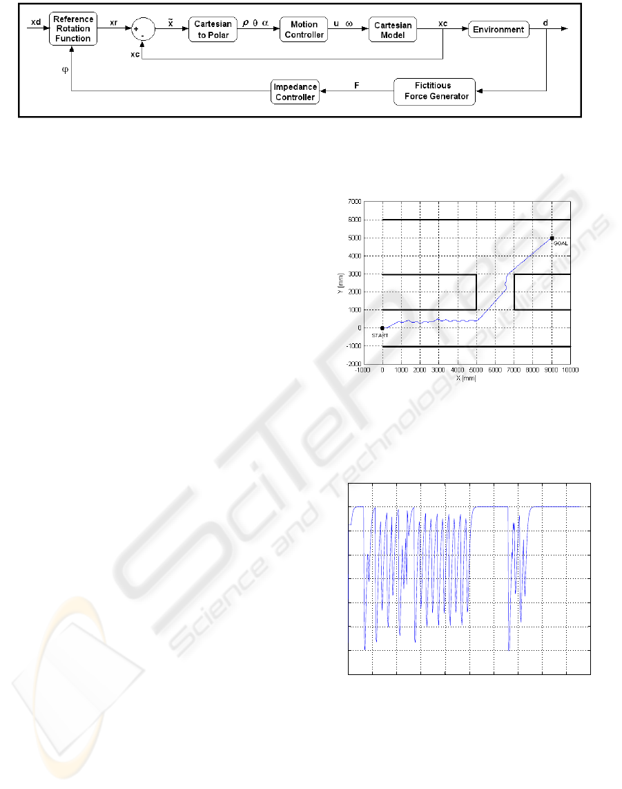
Figure 3: Block diagram corresponding to the Impedance Based Control System.
impedance controller (Hogan, 1985)). The rotation
(avoidance) angle is inversely proportional to the dis-
tance robot-obstacle and to the angle β. In this strat-
egy the path the robot takes to escape from an obstacle
is not taken into account. The vehicle is supposed to
get close to the real target position while maneuver-
ing to avoid any obstacle. After passing the obstacle,
the angle ϕ becomes zero and the rotation matrix be-
comes an identity one, thus causing x
d
not to change.
Finally, it is worthy to emphasize that this control
system is stable in the Lyapunov sense (Secchi et al.,
2001). This means that the robot will always reach
the goal (if the goal is reachable), independently of
the obstacles in its path.
2.2 A Simulated Example
An example is here simulated, in which the ro-
bot should reach the point (9000 mm, 5000 mm),
avoiding any obstacle in its path. Fig. 4 shows the
path followed by the robot from the starting point
(0 mm, 0 mm, 0) to the destination point (the orien-
tation of the robot when reaching the goal is not taken
into account). When an obstacle is detected, a ficti-
tious force is generated and the robot makes a turn.
The value of d
max
was chosen to be 70 cm. Fig. 5
shows the control signal u generated by the final pose
controller. From such figure one can notice meaning-
ful variations in the robot linear velocity. They mean
great acceleration and deceleration of the robot mo-
tors.
3 THE NEW CONTROL SYSTEM
A new control system is here proposed, which is
based in escape paths that are tangent to the obstacle
detected. Such a control system uses just part of the
Impedance Based Control system, namely the inner
loop in Fig. 3 (see Fig. 6). The difference is that the
rotation angle ϕ is not calculated using the repulsive
force F anymore, but using the angular position of
the obstacle relative to the robot. The rotation angle
is now determined to make the vehicle to turn around
Figure 4: The path followed by the robot (Impedance).
0 5 10 15 20 25 30 35 40 45 50
−50
0
50
100
150
200
250
300
350
t [s]
u [mm/s]
Figure 5: The linear velocity of the robot (Impedance).
until getting aligned to the tangent to the obstacle con-
tour. One advantage of this method is that the robot
contours the obstacle, thus describing excellent trajec-
tories when navigating (Maravall and de Lope, 2002),
as it is shown in the sequence.
A NEW APPROACH TO AVOID OBSTACLES IN MOBILE ROBOT NAVIGATION: TANGENTIAL ESCAPE
343
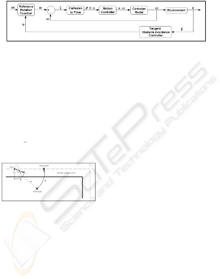
Figure 6: Block diagram corresponding to the new control system.
3.1 Describing the New Control
System
When the robot gets into the repulsion zone (Fig. 7),
the angle β is determined (it is the angle between the
axis of movement of the robot and the radius corre-
sponding to the sensor measuring the least distance
from the robot to the obstacle detected). Knowing the
robot orientation relative to the real target (the angle
α) and the positions of the ultrasonic sensors around
the robot platform, the angle ϕ that allows a tangential
deviation is obtained as
ϕ =
π
2
− |β|
reverseSign(β) − α, (6)
where reverseSign(β) corresponds to −Sign(β).
Figure 7: Obtaining the angle ϕ.
The angle ϕ is then used in the rotation matrix in
(5) and the real target is rotated to a new position (the
virtual target). The final pose controller, which calcu-
lates the new robot orientation to reach the target, uses
the coordinates of the virtual target, causing the robot
to take the tangent to the obstacle border. Notice that
in the absence of obstacles the change in the position
of the real target is null, and the robot continues seek-
ing for the real target. This algorithm is represented
in Fig. 6, where u, ω and the vector x
c
have the same
meaning as in Section 2.
It is important to notice that the control loop cor-
responding to the proposed controller is slower than
the control loop corresponding to the final pose con-
troller. Then, the robot is able to follow the varia-
tion imposed to the target position. Notice also that
the same idea applies to the impedance based con-
trol. Knowing this, the asymptotic stability of the
impedance based control system is demonstrated in
(Secchi et al., 2001). Now, if one compares the block
diagrams corresponding to both impedance based and
tangential deviation control systems, it is possible to
realize that the proposed control system is also as-
ymptotically stable, once the inner loop of both sys-
tems is the same. This means that the strategy here
proposed for obstacle deviation always takes the ro-
bot to the target (if the target is reachable), thanks to
its asymptotic stability.
3.2 A Simulated Example
The objective in this simulation is to take the robot
from the starting point (0 mm, 0 mm, 0) to the goal
point (9000 mm, 5000 mm) once more, avoiding any
obstacle in its path. Fig. 8 shows the path the robot
followed until reaching the goal. As the obstacles (the
walls of the corridors the robot enters in) are detected,
the robot turns around in order to follow a line paral-
lel to the walls. The repulsion zone was defined as
70 cm once more. Fig. 9 shows the linear velocity
developed by the robot. An important remark about
this method is that while avoiding obstacles, approxi-
mately between 4s and 17s in Fig. 9, the robot keeps
navigating with constant linear velocity (the values of
the angular velocity and the orientation, in such time
interval, are very close to zero).
3.3 Comparing the Results
After analyzing the graphics related to the impedance
based control system and the proposed control sys-
tem, it is possible to figure out some strong differ-
ences between both approaches. The first one is
that while avoiding obstacles the strategy here pro-
posed assures constant linear velocity to the robot,
thus avoiding unnecessary acceleration and deceler-
ation, reducing the energy consumption and saving
batteries.
In addition, the tangential obstacle avoidance al-
lows reaching the target point in less time than the
ICINCO 2005 - ROBOTICS AND AUTOMATION
344
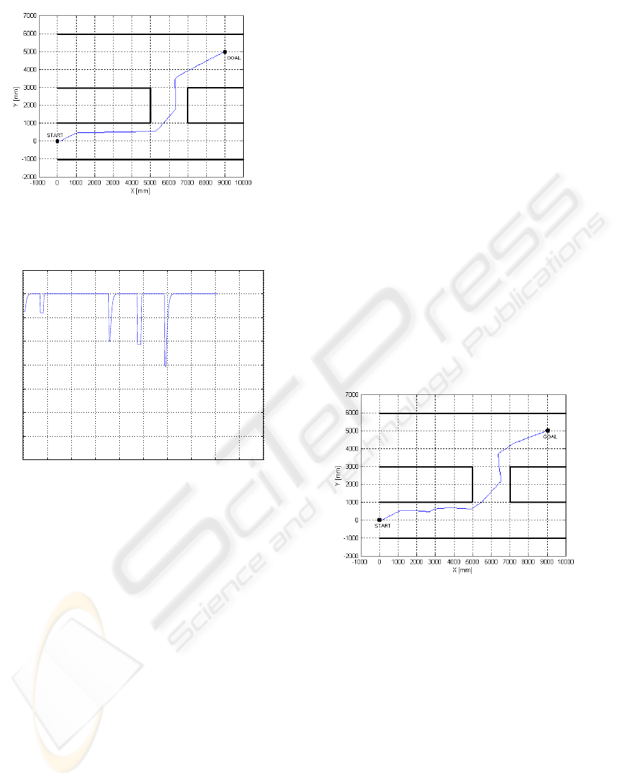
Figure 8: The path followed by the robot (Proposed
Method).
0 5 10 15 20 25 30 35 40 45 50
−50
0
50
100
150
200
250
300
350
t [s]
u [mm/s]
Figure 9: The linear velocity of the robot (Proposed
Method).
impedance based strategy. This is a consequence of
the facts that the path the robot follows is closer to
the optimum one, as one can see in Fig. 8, and the ro-
bot linear velocity is not decreased during the obstacle
avoidance, which occurs when using the impedance
based strategy. Therefore, the strategy here proposed
for obstacle avoidance is extremely attractive.
In addition, the simulated example itself shows that
the tangential strategy for obstacle avoidance gives
the robot the capability of following walls or corri-
dors with no additional computation.
4 EXPERIMENTAL RESULTS
In order to validate the control system here proposed,
it was programmed in the computer onboard the Pi-
oneer 2-DX mobile robot and was tested in various
experiments. One of these experiments corresponds
to the trajectory in Fig. 10, and confirms the ef-
fectiveness of the tangential obstacle avoidance ap-
proach. The robot is supposed to reach the point
(9000 mm, 5000 mm), starting navigating in the
point (0 mm, 0 mm, 0). This experiment confirms
the simulated results, as one can see by comparing the
graphics corresponding to the real experiment and to
the simulation in Section 3.
The second experiment corresponds to a very im-
portant situation (see Fig. 11): due to the position of
of the starting point and the goal, as well as the config-
uration of the walls, the robot is supposed to describe
an U path. In this situation it is forced to overlap the
goal position, because of the wall at its left side, thus
going too far from the goal before restarting seeking
for it again. This point represents a local minimum
and the proposed method allows escaping from situ-
ations like that, as shown in the experiment. As one
can see, it does not gets stuck in a local minimum, like
it happens in connection to the Potential Field method
(and those that are derived from it). The same figure
also shows how the robot performs when there are ob-
stacles in a corridor: the tangential escape approach
makes it to contour the obstacle, like one can see in
Fig. 11.
Figure 10: The path followed by the robot (Proposed
Method).
As one can also see from Fig. 11, the approach pro-
posed to avoid obstacles has been successful in guid-
ing the robot through narrow passages. The two ob-
stacles in the first horizontal and in the vertical cor-
ridors create narrow passages through which the pro-
posed control system guides the robot.
To close the experimentation, the same experi-
ments were also run using the Impedance Based Con-
trol system. In the first one the robot reached the goal
without major problems, but in the second one it did
not manage to go beyond the obstacle in the horizon-
tal corridor. Then, one gets the conclusion that the
proposed approach is effectively much better in terms
of avoiding obstacles, energy consumption, time to
get the goal and motor wearing.
A NEW APPROACH TO AVOID OBSTACLES IN MOBILE ROBOT NAVIGATION: TANGENTIAL ESCAPE
345
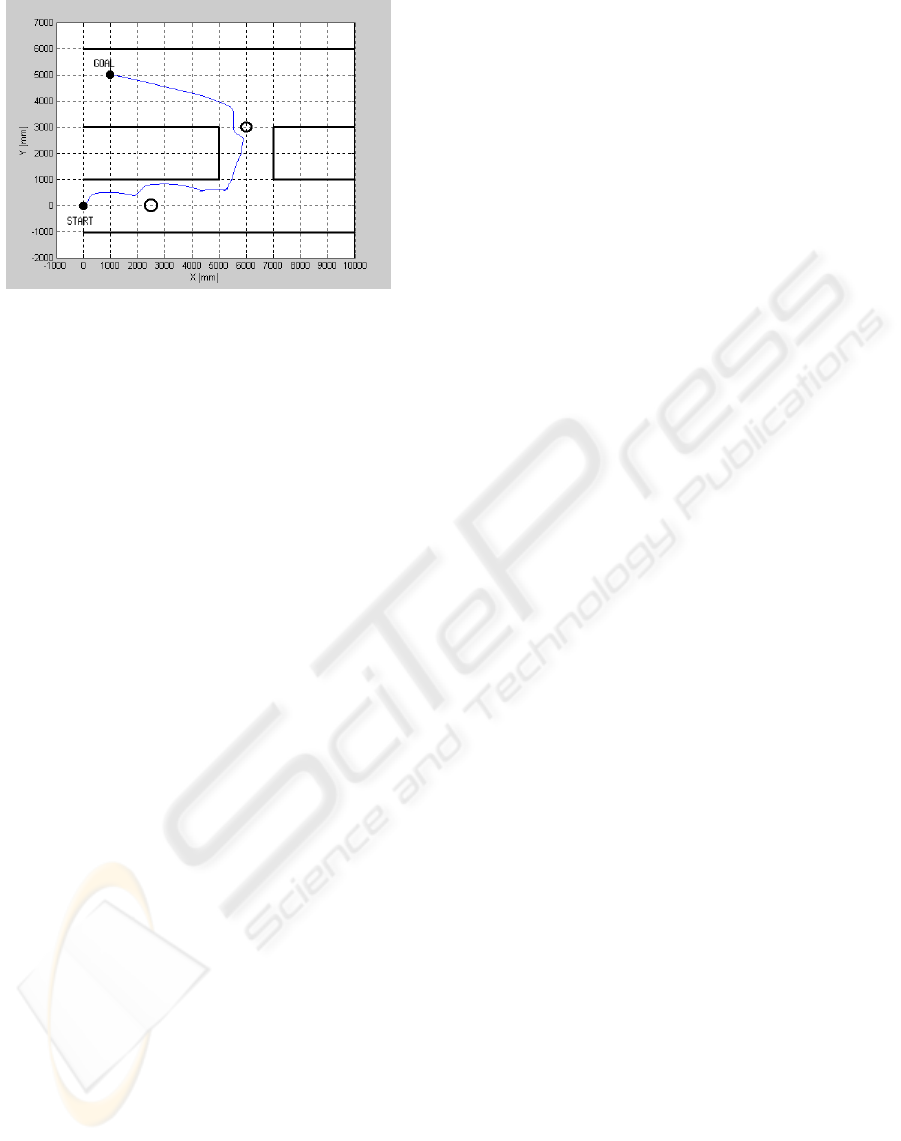
Figure 11: Experiment in a U-path with two obstacles (Pro-
posed Method).
5 CONCLUSION
A new method is proposed in this paper to control a
mobile robot when avoiding obstacles along its path
from a starting point to a target point. Such method
is a modification of the well known Impedance Based
Control System, in which the target point has its real
position temporarily redefined, thus causing a change
in the robot path in order to deviate from any obsta-
cle. The same strategy is here adopted, but the idea is
to redefine the temporary position of the target point
according to a new paradigm: the robot should keep
aligned to the tangent to the obstacle border.
The control system thus implemented is shown
to be stable in the Lyapunov sense, as well as the
impedance based one, and many experiments have
shown its efficiency in guiding the robot. The whole
path followed by the robot is quite close to the optimal
one, the maneuvers performed are softer, the naviga-
tion time is lower and the motors of the mobile robot
are less demanded, for the lower variations imposed to
the angular and linear velocities, as it can be checked
in the experiments presented.
Finally, besides its simplicity and effectiveness, it
should be emphasized that the proposed control sys-
tem also allows implementing the behaviors Wall Fol-
lowing and Corridor Following with no additional
computation.
REFERENCES
Althaus, P. and Christensen, H. I. (2002). Behaviour co-
ordination for navigation in office environments. In
IEEE/RSJ International Conference on Intelligent Ro-
bots and System, volume 3, pages 2298–2304, Lau-
sanne, Switzerland.
Borenstein, J. and Koren, Y. (1989). Real-time obstacle
avoidance for fast mobile robots. IEEE Transactions
on Systems, Man, and Cybernetics, 19(5):1179–1187.
Borenstein, J. and Koren, Y. (1991). The vector field
histogram - fast obstacle avoidance for mobile ro-
bots. IEEE Transactions on Robotics and Automation,
7(3):278–288.
Brock, O. and Khatib, O. (1999). High-speed navigation us-
ing the global dynamic window approach. In Proc. of
the 1999 IEEE International Conference on Robotics
and Automation, volume 1, pages 341–346.
Elfes, A. (1987). Sonar-based real-world mapping and nav-
igation. IEEE Journal of Robotics and Automation,
RA-3(3):249–265.
Fox, D., Burgard, W., and Thrun, S. (1997). The dynamic
window approach to collision avoidance. Robotics &
Automation Magazine, IEEE, 4(1):23–33.
Hogan, N. (1985). Impedance control: An approach to ma-
nipulation. ASME Journal of Dynamic Systems, Mea-
surement, and Control, 107:1–23.
Khatib, O. (1986). Real time obstacle avoidance for manip-
ulators and mobile robots. The International Journal
of Robotics Research, 5(1):90–98.
Kuc, R. and Barshan, B. (1989). Navigating vehicles
through an unstructured environment with sonar. In
Proc. of the 1989 IEEE International Conference on
Robotics and Automation, volume 3, pages 1422–
1426, Scottsdale, AZ.
Maravall, D. and de Lope, J. (2002). Integration of arti-
ficial potential field theory and sensory-based search
in autonomous navigation. In XV World Congress
of the International Federation of Automatic Control,
IFAC’2002, Barcelona, Spain.
Minguez, J. and Montano, L. (2004). Nearness diagram
(nd) navigation: collision avoidance in troublesome
scenarios. IEEE Transactions on Robotics and Au-
tomation, 20(1):45–59.
Secchi, H., Carelli, R., and Mut, V. (2001). Discrete sta-
ble control of mobile robots with obstacles avoidance.
In International Conference on Advanced Robotics,
ICAR’01, pages 405–411, Budapest, Hungary.
ICINCO 2005 - ROBOTICS AND AUTOMATION
346
