
SFM FOR PLANAR SCENES: A DIRECT AND ROBUST APPROACH
∗
Fadi Dornaika and Angel D. Sappa
Computer Vision Center
Edifici O Campus UAB
08193 Bellaterra, Barcelona, Spain
Keywords:
Structure From Motion, motion field, image derivatives, robust statistics, non-linear optimization.
Abstract:
Traditionally, the Structure From Motion (SFM) problem has been solved using feature correspondences. This
approach requires reliably detected and tracked features between images taken from widespread locations. In
this paper, we present a new paradigm to the SFM problem for planar scenes. The novelty of the paradigm
lies in the fact that instead of image feature correspondences, only image derivatives are used. We introduce
two approaches. The first approach estimates the SFM parameters in two steps. The second approach directly
estimates the parameters in one single step. Moreover, for both strategies we introduce the use of robust
statistics in order to get robust solutions in presence of outliers. Experiments on both synthetic and real image
sequences demonstrated the effectiveness of the developed methods.
1 INTRODUCTION
Computing object and camera motions from 2D im-
age sequences has been a central problem in computer
vision for many years. More especially, computing
the camera motion and/or its 3D velocity is of partic-
ular interest to a wide variety of applications in com-
puter vision and robotics such as calibration, visual
servoing, etc. Many algorithms have been proposed
for estimating the 3D relative camera motions (dis-
crete case) (Jonathan et al., 2002; Weng et al., 1993;
Zucchelli et al., 2002) and the 3D velocity (differen-
tial case) (Brooks et al., 1997). The discrete case re-
quires feature matching/tracking, and the differential
case the computation of the optical flow field (2D ve-
locity). These tasks are generally ill-conditioned due
to significant local appearance changes and/or large
disparities. Most of the SFM algorithms are general in
the sense that they assume no prior knowledge about
the scene. In many practical cases, planar or quasi-
planar structures occur frequently in real images. In
this paper, we introduce a novel paradigm to deal with
the SFM problem of planar scenes using image deriv-
atives only. This paradigm has the following advan-
∗
This work was supported in part by the Government
of Spain under the CICYT project TRA2004-06702/AUT;
both authors were supported by The Ram
´
on y Cajal Pro-
gram.
tages. First, we need not to extract features nor to
track them in several images. Second, robust statis-
tics are invoked in order to get stable estimates. We
introduce two approaches. The first approach esti-
mates the SFM parameters in two steps. The second
approach directly estimates the parameters in one sin-
gle step. Using image derivatives has been exploited
in (Brodsky and Fermuller, 2002) to make camera in-
trinsic calibration. In our study, we deal with the 3D
motion of the camera as well as with the plane struc-
ture. The paper is organized as follows. Section 2
states the problem. Section 3 describes a two-step
approach. Section 4 describes a one-step approach.
Section 5 shows how image derivatives are computed.
Experimental results on both synthetic and real image
sequences are given in Section 6.
2 BACKGROUND
Throughout this paper we represent the coordinates
of a point in the image plane by small letters (x, y)
and the object coordinates in the camera coordinate
frame by capital letters (X, Y, Z). In our work we
use the perspective camera model as our projection
model. Thus, the projection is governed by the fol-
lowing equation were the coordinates are expressed
175
Dornaika F. and D. Sappa A. (2005).
SFM FOR PLANAR SCENES: A DIRECT AND ROBUST APPROACH.
In Proceedings of the Second International Conference on Informatics in Control, Automation and Robotics - Robotics and Automation, pages 175-180
DOI: 10.5220/0001173801750180
Copyright
c
SciTePress
in homogeneous form,
λ
x
y
1
!
=
f s f x
0
0 γ f y
0
0 0 1
!
X
Y
Z
1
(1)
Here, f denotes the focal length in pixels, γ and s
the aspect ratio and the skew and (x
0
, y
0
) the prin-
cipal point. These are called the intrinsic parame-
ters. In this study, we assume that the camera is cal-
ibrated, i.e., the intrinsic parameters are known. For
the sake of presentation simplicity, we assume that the
image coordinates have been corrected for the princi-
pal point and the aspect ratio. This means that the
camera equation can be written as in (1) with γ = 1,
and (x
0
, y
0
) = (0, 0). Also, we assume that the skew
is zero (s = 0). With these parameters the projection
simply becomes
x = f
X
Z
and y = f
Y
Z
(2)
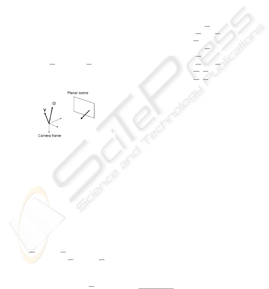
Figure 1: The goal is to compute the camera 3D velocity as
well as the plane structure from the image derivatives.
Let I(x, y, t) be the intensity at pixel (x, y) in the
image plane at time t. Let u(x, y) and v(x, y) de-
note components of the motion field in the x and y
directions respectively. This motion field is caused
by the translational and rotational camera velocities
(V, Ω) = (V
x
, V
y
, V
z
, Ω
x
, Ω
y
, Ω
z
). Using the con-
straint that the gray-level intensity is locally invariant
to the viewing angle and distance we obtain the well-
known optical flow constraint equation:
I
x
u + I
y
v + I
t
= 0 (3)
where u =
∂x
∂t
and v =
∂y
∂t
denote the motion field.
The spatial derivatives I
x
=
∂I
∂x
and I
y
=
∂I
∂y
(the im-
age gradient components) can be computed by convo-
lution with derivatives of a 2D Gaussian kernel. They
can be computed from one single image - the current
image. The temporal derivative I
t
=
∂I
∂t
can be com-
puted by convolution between the derivative of a 1D
Gaussian and the image sequence (see Section 5).
The perspective camera observes a planar scene
2
described in the camera coordinate system by Z =
A X + B Y + C.
One can show that the equations of the motion field
as a function of the 3D velocity (V, Ω) are given by
these two equations:
u(x, y) = a
1
+ a
2
x + a
3
y + a
7
x
2
+ a
8
xy(4)
v(x, y) = a
4
+ a
5
x + a
6
y + a
7
xy + a
8
y
2
(5)
where the coefficients are depending on the SFM pa-
rameters:
a
1
= −f (
V
x
C
+ Ω
y
)
a
2
= (
V
x
C
A +
V
z
C
)
a
3
=
V
x
C
B + Ω
z
a
4
= −f (
V
y
C
− Ω
x
)
a
5
= (
V
y
C
A − Ω
z
)
a
6
= (
V
y
C
B +
V
z
C
)
a
7
=
−1
f
(
V
z
C
A + Ω
y
)
a
8
=
−1
f
(
V
z
C
B − Ω
x
)
(6)
One can notice that the two solutions (V
x
, V
y
, V
z
, C)
and λ (V
x
, V
y
, V
z
, C) yield the same motion field.
This is consistent with the scale ambiguity that occurs
in the general SFM problem.
Our goal is to estimate the instantaneous camera
velocity (V, Ω) as well as the plane orientation from
the image derivatives. The translational velocity can
be recovered up to a scale. It should be noticed that
for continuous videos the camera motion has to be
computed for all time instants during which the cam-
era is moving.
3 A TWO-STEP APPROACH
In this section, we propose a two-step approach. In
the first step, the 8 coefficients (a
1
, . . . , a
8
) are recov-
ered by solving an over-constrained system derived
from (3) using robust statistics. In the second step,
the translational and rotational velocities as well as
the plane orientation are recovered from Eq.(6) using
some non-linear technique.
3.1 Robust Estimation Of The 8
Coefficients
We assume that the image contains N pixels for
which the spatio-temporal derivatives (I
x
, I
y
, I
t
)
have been computed. In practice, N is very large. In
2
Our work also addresses the case where the scene con-
tains a dominant planar structure.
ICINCO 2005 - ROBOTICS AND AUTOMATION
176

order to reduce this number, one can drop pixels hav-
ing small gradient components since they do not have
a heavy impact on the whole accuracy of the solution.
In the sequel, we do not distinguish between the two
cases. By inserting Eqs.(4) and (5) into Eq.(3) we get
I
x
a
1
+ I
x
x a
2
+ I
x
y a
3
+ I
y
a
4
+ I
y
x a
5
+ I
y
y a
6
+(I
x
x
2
+ I
y
x y) a
7
+ (I
x
x y + I
y
y
2
) a
8
= −I
t
(7)
By concatenating the above equation for all pixels,
we get an over-constrained linear system having the
following form:
Ga = e (8)
where a denotes the column vector
(a
1
, a
2
, a
3
, a
4
, a
5
, a
6
, a
7
, a
8
)
T
.
It is well known that the Maximum Likelihood so-
lution to the above linear system is given by:
a = G
†
e (9)
where G
†
= (G
T
G)
−1
G
T
is the pseudo-inverse of
the N × 8 matrix G. This solution is known as the
Least Square solution (LS). The above solution is
only optimal in the case where the linear system is
corrupted by Gaussian noise with a fixed variance.
In practice, the system of linear equations may con-
tain outliers. In other words, there are some pixels
for which the residual of Eq.(3) is very large and can
affect the solution. These outliers can be caused by
local planar excursions and derivatives errors. There-
fore, our idea is to estimate the 8 coefficients using
robust statistics (Huber, 2003). We proceed as fol-
lows. First, equations are explored using subsamples
of p linear equations (remember that each linear equa-
tion in (8) is provided by a pixel). For the problem at
hand, p should be at least eight. Second, the solution
is chosen according to the consensus measure based
on residual errors. A Monte Carlo type technique
is used to draw K random subsamples of p different
equations/pixels. Figure 2 illustrates the algorithm.
Detecting inliers The question now is: Given a sub-
sample k and its associated solution a
k
, How do we
decide whether or not a pixel is an inlier? In tech-
niques dealing with geometrical features (points and
lines) (Fischler and Bolles, 1981), this can be easily
achieved using the distance in the image plane be-
tween the actual location of the feature and its mapped
location. If this distance is below a given threshold
then this feature is considered as an inlier; otherwise,
it is considered as an outlier.
In our case, however, there are no geometrical fea-
tures at all since only image derivatives are used.
Therefore, our idea is to compute a robust estimation
of standard deviation of the residual errors. In the ex-
ploration step, for each subsample k, the median of
residuals was computed. If we denote by
M the least
Random sampling: Repeat the following three steps
K times
1. Draw a random subsample of p different equa-
tions/pixels.
2. For this subsample, indexed by k, compute the eight co-
efficients, i.e. the vector a
k
, from the corresponding p
equations using a linear system similar to (8).
3. For this solution a
k
, determine the median M
k
of the
squared residuals with respect to the whole set of N
equations. Note that we have N residuals correspond-
ing to the linear system (8).
Consensus step:
1. For each solution a
k
, k = 1, . . . , K, compute the num-
ber of inliers among the entire set of equations/pixels (see
below). Let n
k
be this number.
2. Choose the solution that has the highest number
of inliers. Let a
i
be this solution where i =
arg max
k
(n
k
), k = 1, . . . , K
3. Refine a
i
using the system formed by its inliers, that is,
(9) is used without the outliers.
Figure 2: Recovering the eight coefficients using robust sta-
tistics.
median, then a robust estimation of the standard de-
viation of the residual is given by (Rousseeuw and
Leroy, 1987):
ˆσ = 1.4826
1 +
5
N − p
p
M (10)
Once ˆσ is known, any pixel j can be considered as
an inlier if its residual error satisfies |r
j
| < 3 ˆσ.
The number of subsamples K A subsample is
“good” if it consists of p good pixels. The number
of subsamples is chosen such that the probability P
r
that at least one of the K subsamples is good is very
close to one (e.g., P
r
= 0.98). Assuming that the
whole set of equations may contain up to a fraction ǫ
of outliers, the probability that at least one of the K
subsamples is good is given by
P
r
= 1 − [1 − (1 −ǫ)
p
]
K
Given a prior knowledge about the percentage of out-
liers ǫ the corresponding K can be computed by:
K =
log (1 − P
r
)
log (1 − (1 −ǫ)
p
)
For example, when p = 20, P
r
= 0.98, and ǫ = 20%
we get K = 337 samples.
3.2 The SFM Parameters
Once the eight coefficients are recovered, it
can be shown that the SFM parameters, i.e.
SFM FOR PLANAR SCENES: A DIRECT AND ROBUST APPROACH
177
V
x
C
,
V
y
C
,
V
z
C
, Ω
x
, Ω
y
, Ω
z
, A, and B, can be recov-
ered by solving the non-linear equations (6). This
is carried out using the Levenberg-Marquardt tech-
nique (Press et al., 1992). Non-linear algorithms need
an initial solution. In order to get such initial solutions
one can adopt assumptions for which Eq.(6) becomes
linear. Then, the linear solution is refined using the
Levenberg-Marquardt technique. In practice, one can
use one of the following two assumptions for which
Eq.(6) becomes linear in the parameters:
1. Assume that the translational velocity of the cam-
era along its optical axis is very small compared
to its lateral velocity, that is,
V
z
V
x
<< 1 and/or
V
z
V
y
<< 1. With this assumption, we can set V
z
to 0 in Eq.(6) which can be easily solved for the
remaining parameters.
2. Assume that the camera motion is a pure transla-
tion, then compute the translation velocity and the
plane orientation using the resulting linear system.
We point out that the discrepancy between the linear
solution and the true one depends on the realism of
the made assumption.
4 A ONE-STEP APPROACH
In this section, we propose a second approach that
directly estimates the SFM parameters in one single
step. To this end, Eqs.(4), (5), and (6) are inserted into
Eq.(3). The result is a system with N non-linear equa-
tions relating the unknowns to the image derivatives.
This can be solved using the Levenberg-Marquardt
technique. For each pixel i, Equation (3) gives a non-
linear constraint having the form f
i
= 0. Thus, the
SFM parameters are obtained by minimizing the fol-
lowing cost function:
min
b
N
X
i=1
f
2
i
(11)
where b = (
V
x
C
,
V
y
C
,
V
z
C
, Ω
x
, Ω
y
, Ω
z
, A, B)
T
.
The robust version of the one-step approach is ob-
tained from Eq. (11) by retaining only the inlier pix-
els:
min
b
N
X
i=1
w
i
f
2
i
, w
i
=
1 if the pixel i is inlier
0 otherwise
The detection of inlier pixels is performed using the
paradigm described in Section 3.1.
This approach provides a direct estimation of the
unknowns from the image derivatives and is expected
to be more accurate than the two-step approach (see
experiments below). Indeed, in the two-step ap-
proach, errors associated the estimated 8 coefficients
a will affect the estimation of the SFM parameters in
the second step - solving Eq. (6).
5 THE DERIVATIVES
The spatial derivatives associated with the current im-
age are calculated by convolution with derivatives of
2D Gaussian kernels. That is, I
x
= I ∗ G
x
and
I
y
= I ∗ G
y
where
G
x
= −
1
2πσ
4
s
x exp
−
x
2
+ y
2
2σ
2
s
(12)
G
y
= −
1
2πσ
4
s
y exp
−
x
2
+ y
2
2σ
2
s
(13)
The temporal derivatives associated with the current
image are calculated using difference approximation
involving a temporal window centered on the current
image. The weights of the images are taken from the
derivatives of a 1D Gaussian kernel. That is, I
t
=
I ∗ G
t
where
G
t
= −
1
√
2πσ
3
t
t exp
−
t
2
2σ
2
t
(14)
The images can be smoothed before computing the
temporal derivatives using Gaussian kernels having
the same spatial scale σ
s
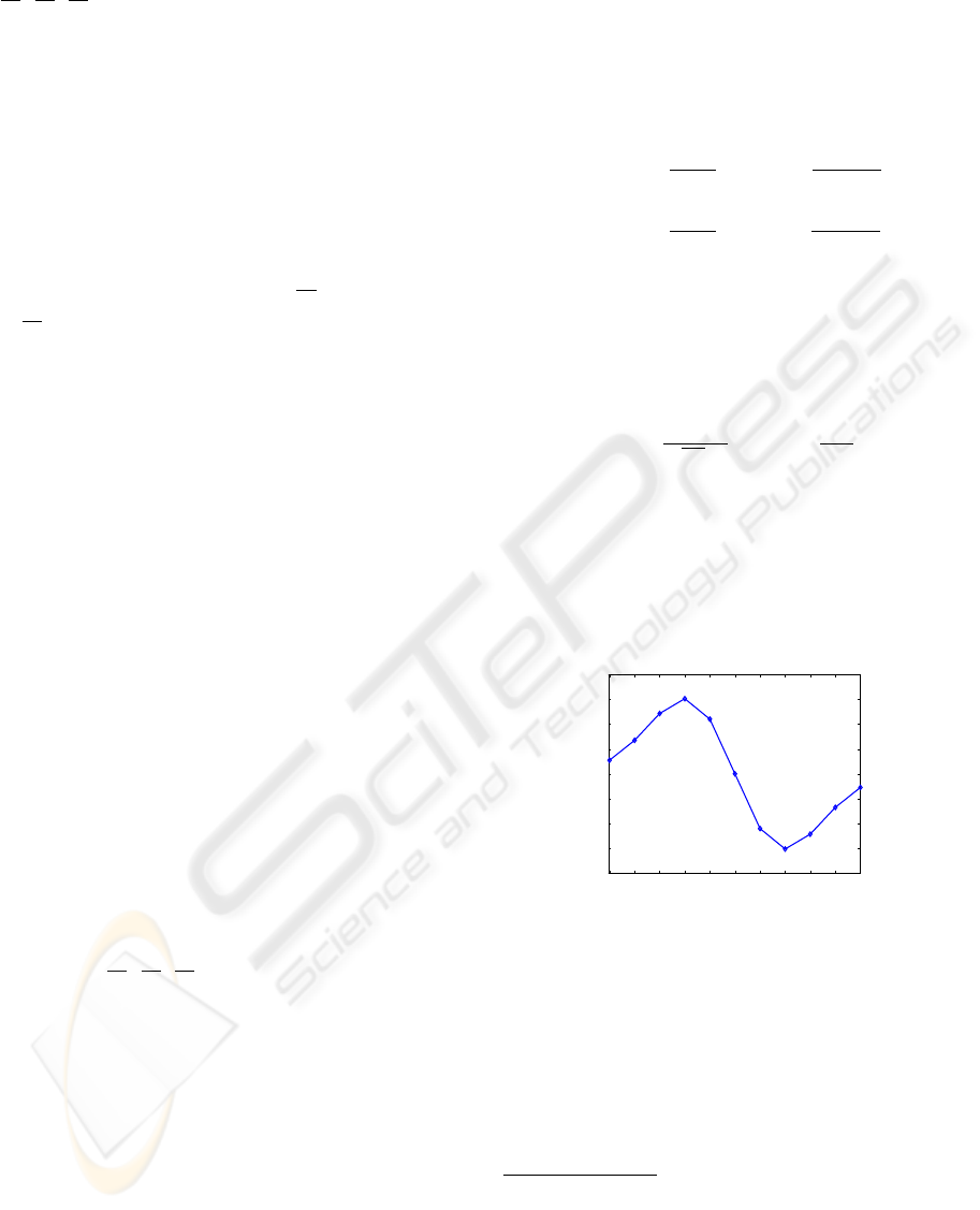
. Figure 3 shows 11 weights
approximating G
t
whose σ
t
is set to 2 frames. These
weights correspond to 11 subsequent images. The
smoothness achieved by the spatial and the temporal
Gaussians is controlled by σ
s
and σ
t
, respectively.
−5 −4 −3 −2 −1 0 1 2 3 4 5
−0.08
−0.06
−0.04
−0.02
0
0.02
0.04
0.06
0.08
Images
Figure 3: The 11 weights approximating the derivatives of
1D Gaussian whose σ
t
is set to 2 frames.
6 EXPERIMENTS
Experiments have been carried out on synthetic and
real images.
Synthetic images
Experiments have been carried out
on synthetic images featuring planar scenes. The tex-
ture of the scene is described by:
g(X
o
, Y
o
) = sin(c
h
X
o
) + sin(c
v
Y
o
)
where X
o
and Y
o
are the 3D coordinates expressed in
the plane coordinates system, see Figure 4. The res-
olution of the synthesized images is 160×160 pixels.
ICINCO 2005 - ROBOTICS AND AUTOMATION
178
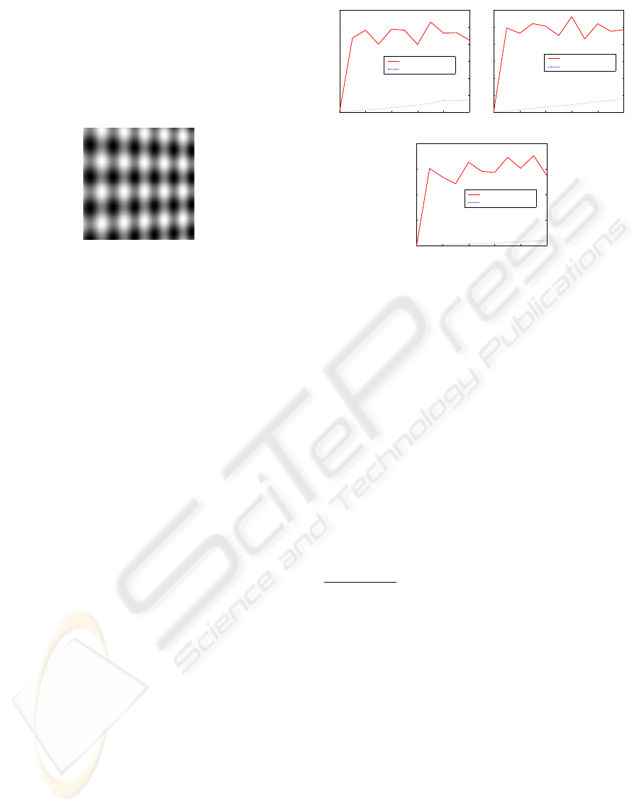
The constants c
h
and c
v
control the periodicity of the
sine waves along each direction (in our example, these
constants are set to 1.5). The 3D plane was placed at
100cm from the camera whose focal length is set to
1000 pixels. In order to study the performance of the
developed approaches, we have proposed the follow-
ing framework.
Figure 4: A computer generated image of a 3D plane. The
plane is rotated about 40 degrees about the fronto-parallel
plane.
A synthesized image sequence of the planar scene
is generated according to a nominal camera veloc-
ity (V
n
, Ω
n
). A reference image is then fixed for
which the image derivatives are computed and for
which we like to compute the SFM parameters. Since
synthetic data are used ground-truth values for the
image derivatives and for the SFM parameters are
known. The nominal 3D velocity (V
n
, Ω
n
) is set
to (10cm/s, 10, 1, 0.1rad/s, 0.1, 0.1)
T
. The corre-
sponding linear system (8) is then gradually corrupted
by a Gaussian noise having an increasing variance.
Our approach is then used to solve the SFM problem
using the corrupted linear system. The discrepancies
between the estimated parameters and their ground
truth are then evaluated. In our case, the SFM pa-
rameters are given by three vectors (see Figure 1): the
scaled translational velocity, (ii) the rotational veloc-
ity, and (iii) the plane normal in the camera coordinate
system. Thus, the accuracy of estimated parameters
can be summarized by the angle between the direction
of the estimated vector and its ground truth direction.
The goal is to quantify the accuracy of the two-step
approach (Section 3). To this end, the simulated lin-
ear system was corrupted by a pure Gaussian noise as
well as by a 15% of outliers. The standard deviation
of the Gaussian noise is gradually increased as a per-
centage of the mean of the spatio-temporal derivatives
(ground truth values). The outliers are uniformly se-
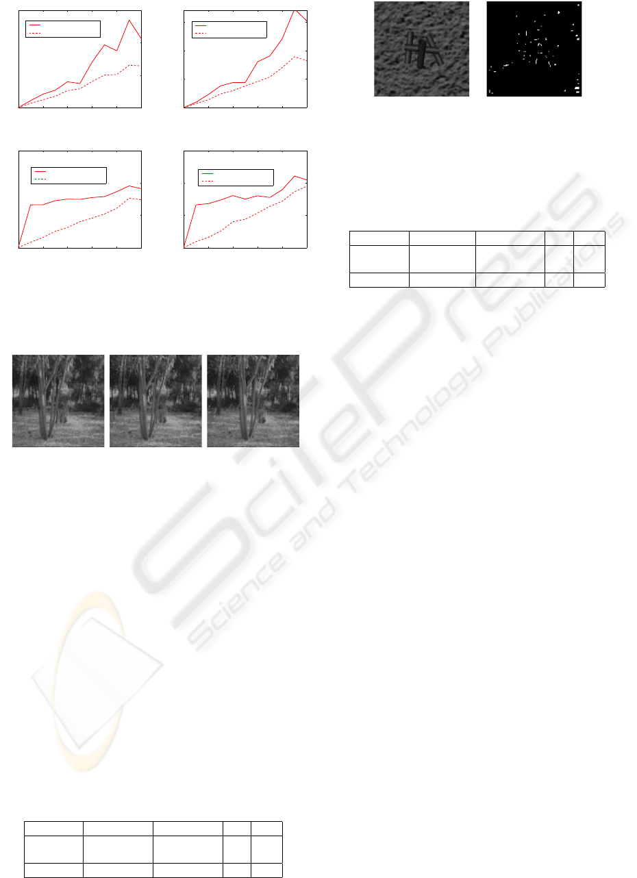
lected in the image. Figure 5 illustrates the obtained
average errors associated with the SFM parameters as
a function of the Gaussian noise (using the two-step
approach). The solid curve corresponds to the Least
Square solution (no robust statistics), and the dotted
curve to the robust solution. In this figure, each aver-
age error was computed with 50 random realizations.
As can be seen, unlike the LS solution the second so-
lution is much more accurate.
0 2 4 6 8 10
0
10
20
30
40
50
60
Noise percentage (standard deviation)
Average error (Deg.)
Translational velocity
LS solution
Robust solution
0 2 4 6 8 10
0
10
20
30
40
50
60
Noise percentage (standard deviation)
Average error (Deg.)
Rotational velocity
LS solution
Robust solution
0 2 4 6 8 10
0
5
10
15
20
Noise percentage (standard deviation)
Average error (Deg.)
Plane orientation
LS solution
Robust solution
Figure 5: Average errors associated with the SFM parame-
ters when the system is corrupted by both a Gaussian noise
and 15 % of outliers.
Two-step approach versus one-step approach
Figure 6.(a) shows the average errors associated with
the translational and rotational velocities as a function
of a pure Gaussian noise. The solid curve corresponds
to the two-step approach (Section 3) and the dashed
curve corresponds to the one-step approach (Section
4). Figure 6.(b) shows the same comparison when
both Gaussian noise and outliers are added. As can
be seen, the second approach seems to be more ac-
curate than the first one. This behavior holds for the
plane orientation.
Real images
The first experiment was conducted
on a video sequence captured by a moving cam-
era, see Figure 7. This video was retrieved from
ftp://csd.uwo.ca/pub/vision. We have
used 11 subsequent images to compute the SFM
parameters associated with the central image (frame
6). The results are summarized in Table 1. The first
row corresponds to the LS solution (the two-step
approach), the second row to the robust solution
(the two-step approach), and the third row to the
one-step approach. As can be seen, the motion is
essentially a lateral motion. Note the consistency of
the results obtained by the three methods. The second
experiment was conducted on the sequence depicted
in Figure 8.(a). The sequence was retrieved from
http://www.cee.hw.ac.uk/˜mtc/sofa.
The obtained results are summarized in Table 2. As
can be seen, the camera velocity is a rotation about
the optical axis combined with a translation about
the same axis. Figure 8.(b) shows the map of outlier
pixels.
SFM FOR PLANAR SCENES: A DIRECT AND ROBUST APPROACH
179
0 2 4 6 8 10
0
5
10
15
Noise percentage (standard deviation)
Average error (Deg.)
Translational velocity
Two−step method
One−step method
0 2 4 6 8 10
0
5
10
15
Noise percentage (standard deviation)
Average error (Deg.)
Translational velocity
Two−step method
One−step method
0 2 4 6 8 10
0
5
10
15
Noise percentage (standard deviation)
Average error (Deg.)
Rotational velocity
Two−step method
One−step method
0 2 4 6 8 10
0
5
10
15
Noise percentage (standard deviation)
Average error (Deg.)
Rotational velocity
Two−step method
One−step method
(a) (b)
Figure 6: Two-step approach (solid curve) versus the one-
step approach (dashed curve). (a) Gaussian noise. (b)
Gaussian noise and outliers.
frame 1 frame 6 frame 11
Figure 7: The first experiment. Frame 6 represents the cur-
rent image for which the SFM parameters are computed.
The temporal derivatives are computed using 11 subsequent
images.
7 CONCLUSION
We presented a novel paradigm for the planar SFM
problem where only image derivatives have been
used. No feature extraction or matching is needed us-
ing this paradigm. Two different strategies have been
proposed. The first strategy estimates the parameters
of the 2D motion field then the SFM parameters. The
second strategy directly estimates the SFM parame-
ters. Methods from robust statistics were included
in both strategies in order to get an accurate solution
even when data contain outliers. This is very useful
for scenes which are not fully described by planar sur-
Table 1: Results of the first experiment.
Translation Rotation A B
LS sol. (-.99,-.12,.01) (-.13,.99,-.01) .04 -.01
Robust sol. (-.98,-.17,.01) (-.18,.98,-.01) .04 -.01
One step (-.98,-.18,.01) (-.17,.98,-.01) .04 -.00
(a) (b)
Figure 8: The second experiment. (a) The current image
for which the SFM parameters are computed. The temporal
derivatives are computed using 7 subsequent images. (b)
The map of outlier pixels.
Table 2: Results of the second experiment.
Translation Rotation A B
LS sol. (.00,13,.99) (.11,.0,-.99) .34 -1.
Robust sol. (-.01,.08,.99) (.07,.0,-.99) .46 -.89
One step (.14,.08,.98) (.07,-.12,-.98) .55 -.15
faces. The developed strategies do not rely on pixel
velocities. However, these velocities are a byproduct
of them. Future work would be the simultaneous SFM
estimation and camera self-calibration.
REFERENCES
Brodsky, T. and Fermuller, C. (2002). Self-calibration from
image derivatives. International Journal of Computer
Vision, 48(2):91–114.
Brooks, M., Chojnacki, W., and Baumela, L. (1997). Deter-
mining the egomotion of an uncalibrated camera from
instantaneous optical flow. Journal of the Optical So-
ciety of America A, 14(10):2670–2677.
Fischler, M. and Bolles, R. (1981). Random sample consen-
sus: A paradigm for model fitting with applications to
image analysis and automated cartography. Commu-
nication ACM, 24(6):381–395.
Huber, P. (2003). Robust Statistics. Wiley.
Jonathan, A., M., and Sclaroff, S. (2002). Recursive esti-
mation of motion and planar structure. In IEEE Con-
ference on Computer Vision and Pattern Recognition.
Press, W. H., Teukolsky, S. A., Vetterling, W. T., and Flan-
nery, B. P. (1992). Numerical Recipes in C. Cam-
bridge University Press.
Rousseeuw, P. and Leroy, A. (1987). Robust Regression and
Outlier Detection. John Wiley & Sons, New York.
Weng, J., Huang, T. S., and Ahuja, N. (1993). Motion and
Structure from Image Sequences. Springer-Verlag,
Berlin.
Zucchelli, M., Jose, S., and Christensen, H. (2002). Multi-
ple plane segmentation using optical flow. In British
Machine Vision Conference.
ICINCO 2005 - ROBOTICS AND AUTOMATION
180
