A NEW FAMILY OF CONTROLLERS FOR POSITION CONTROL

ROBOT MANIPULATORS

∗

Fernando Reyes, Jaime Cid, Marco Mendoza, Isela Bonilla

Benem

erita Universidad Aut

onoma de Puebla

Grupo de Rob

otica, Facultad de Ciencias de la Electr

onica

Apartado Postal 542, Puebla 72001, M

exico

Keywords:

Lyapunov function, Global asymptotic stability, PD and PID controllers, Direct-drive robots, position control.

Abstract:

This paper addresses the problem of position control for robot manipulators. A new family of position con-

trollers with gravity compensation for the global position of robots manipulators is presented. The previous

results on the linear PD controller are extended to the new proposed family. The main contribution of this

paper is to prove that the closed–loop system composed by full nonlinear robot dynamics and the family of

controllers is globally asymptotically stable in agreement with Lyapunov’s direct method and LaSalle’s in-

variance principle. Besides the theoretical results, a real-time experimental comparison is also presented on

visual servoing applications to illustrate the performance of the proposed family on a direct–drive robot of two

degrees of freedom.

1 INTRODUCTION

The position control of robot manipulators, or also the

so-called regulation problem is the simplest aim in ro-

bot control and at the same time one of the most rele-

vant issue in practice of manipulators. This is a partic-

ular case of the motion control or trajectory control.

The primary goal of motion control in joint space is to

make the robot joints track a given time-varying de-

sired joint position. On the other hand, the goal of

position control is to move the robot end-effector to

a ﬁxed desired target, which is assumed to be con-

stant, regardless of its initial joint position (Craig,

1989)(F. L. Lewis, 1993)(O. Khatib, 1989).

The PD control is the most widely used strategy

for robot manipulators, because of its simplicity, it

counts with theoretical support to justify the use of the

PD in global positioning (M. Takegaki, 1981)(S. Ari-

moto, 1986)(C. Canudas, 1996). On the other hand,

the PID control is another popular strategy, until now

we do not have the required theoretical support back-

ing to guarantee position control in a global sense

(Kelly, 1995)(R. Kelly, 1996)(Kelly, 1999)(Y. Xu,

1995)(V. Santiba

nez, 1998).

However, the PD control with gravity compen-

sation has serious practical drawback, for example:

∗

Work partially supported by VIEP-BUAP III-66-04

ING/G MEXICO

it requires the exact knowledge of the gravitational

torque vector from robot dynamics. Although the

structure of the gravitational torque vector can be eas-

ily obtained as the gradient of the robot potential en-

ergy due to gravity, some parameters can be uncertain

such as masses and mass centers. Other draws is that

the choice of the PD gains relies on the desired posi-

tion (J. Alvarez, 2003)(A. Loria, 2002)(L. Sciavicco,

1996).

In recent years, various PD-Type control schemes

have been developed for position control of robot ma-

nipulators. Among them the following can be cited: A

PD controller with proportional and derivative gains

as nonlinear functions of the robot states developed

in (Y. Xu, 1995). In the reference (V. Santiba

nez,

1998) was proposed a Saturated PD controller to de-

liver torques within prescribed limits according to the

actuator capability. A new class of nonlinear PID

controllers with robotic applications was presented in

(Seraji, 1998). (Kelly, 1999) presented a PD con-

troller in generic task space. This controller was

based on energy shaping methodology. Most recently,

(J. Alvarez, 2003) proposed a saturated linear PID

controller with semiglobal stability.

In view of the simplicity and applicability of the

simple PD controller in industrial applications, the

main motivation of this paper is in the theoretical and

practical interest of obtaining controllers that lead to

361

Reyes F., Cid J., Mendoza M. and Bonilla I. (2005).

A NEW FAMILY OF CONTROLLERS FOR POSITION CONTROL OF ROBOT MANIPULATORS.

In Proceedings of the Second International Conference on Informatics in Control, Automation and Robotics - Robotics and Automation, pages 361-366

DOI: 10.5220/0001174803610366

 SciTePress

global asymptotic stability of the closed-loop system.

The objective of this paper is to extend the previous

results on the linear PD controller to a new family of

position controllers. In addition to the theoretical is-

sues of the proposed family, this paper also presents

real-time experiments for position control on a direct-

drive robot of two degrees of freedom.

This paper is organized as follows. Section 2 re-

calls the robot dynamics and useful property for sta-

bility proof. In the Section 3, the new family of posi-

tion controllers and its analysis of global asymptotic

stability is presented. Section 4 summarizes the main

components of the experimental set-up. Section 5

contains the experimental results. Finally, some con-

clusions are offered in Section 6.

2 ROBOT DYNAMICS

The dynamics of a serial n-link rigid robot can be

written as (L. Sciavicco, 1996)(Vidyasagar, 1989):

M(q)

q + C(q,

q + g(q) + f (

q, τ ) = τ (1)

where q is the n × 1 vector of joint displacements;

is the n × 1 vector of joint velocities; τ is the n × 1

vector of input torques; M(q) is the n × n symmetric

positive deﬁnite inertia matrix, C(q,

q) is the n × n

matrix of centripetal and Coriolis torques; g(q) is the

n × 1 vector of gravitational torques and f (

q, τ ) is

the n × 1 vector for the friction torques. The vector

q, τ ) is decentralized in the sense that f (

q, τ )

depends only on ˙q

and τ

; that is,

f (

q, τ ) =

( ˙q

, τ

)

( ˙q

, τ

)

( ˙q

, τ

)

The friction torques f(

q, τ ) are assumed to

be dissipate energy at all non-zero velocities, and

therefore, their entries are bounded within the ﬁrst

and third quadrants. This feature allows to consider

the Coulomb and viscous friction common models.

At zero velocities, only static friction is present

satisfying:

(0, τ

) = τ

− g

(q)

for -

≤ τ

− g

(q) ≤

, with

being the limit on

the static friction torques for joint i (B. Armstrong-

elouvry, 1999)(Armstrong-Ho

elouvry, 1991).

It is assumed that the robot links are joined

together with revolute joints. Although the equation

of motion (1) is complex, it has several fundamental

properties which can be exploited to facilitate control

system design. For the new controller, the following

important property is used:

Property 1. The matrix C(q,

q) and the time deriv-

ative

M(q) of the inertia matrix satisfy (Vidyasagar,

1989)(Koditschek, 1984):

M(q) − C(q,

q = 0 ∀ q,

q ∈ IR

. (2)

3 A NEW FAMILY POSITION

CONTROLLERS

This section presents the new family of controllers and its

stability analysis. Consider the following control scheme

with gravity compensation given by

τ = ∇U(K

q) − f

q) + g(q) (3)

where

q = q

− q ∈ IR

is the position error vec-

tor, q

∈ IR

is the desired joint position vector,

∈ IR

n×n

is the proportional gain which is diag-

onal matrix, K

∈ IR

n×n

is a positive deﬁnite matrix,

also called derivative gain, U(K

q) represents the ar-

tiﬁcial potential energy, positive de- ﬁnite function,

and f

q) denotes the damping function, which

is dissipative function, that is,

q) > 0.

The control problem can be stated by selecting the

design functions U(K

q) and f

q) such that the

position error

q and the joint velocity

q vanish asymp-

totically, i.e.,

lim

t→∞

[

q(t),

q(t)]

= 0 ∈ IR

Proposition. Consider the robot dynamic model (1)

together with the control law (3), then the closed-loop

system is globally asymptotically stable and the posi-

tioning aim lim

t→∞

q(t) = q

∧ lim

t→∞

q(t) = 0 is

achieved.

Proof: The closed-loop system equation obtained by

combining the robot dynamic model (1) and control

scheme (3) can be written as

−

−1

(q) [∇U(K

q) − f

−C(q,

(4)

which is an autonomous differential equation, and

the origin of the state space is its unique equilibrium

point.

ICINCO 2005 - ROBOTICS AND AUTOMATION

362

To carry out the stability analysis of equation (4),

the following Lyapunov function candidate is pro-

posed:

V (

q) =

M(q)

q + U(K

q). (5)

The ﬁrst term of V (

q) is a positive deﬁnite func-

tion with respect to

q because M (q) is a positive def-

inite matrix. The second one of Lyapunov function

candidate (5), which can be interpreted as a potential

energy induced by the control law, also is a positive

deﬁnite function with respect to position error

q, be-

cause terms K

and K

are positive deﬁne matrixes.

Therefore, V (

q) is a globally positive deﬁnite and

radially unbounded function.

The time derivative of Lyapunov function candi-

date (5) along the trajectories of the closed-loop equa-

tion (4) and after some algebra and considering prop-

erty 1, can be written as:

V (

q) =

M(q)

q +

M(q)

q − ∇U (K

∇U(K

q) −

q) − C(

q, q)

M(q)

q − ∇U (K

= −

q) ≤ 0, (6)

which is a globally negative semideﬁnite func-

tion and therefore, it is possible to conclude sta-

bility of the equilibrium point. In order to prove

global asymptotic stability, the autonomous nature of

the closed-loop equation (4) is exploited to apply

the LaSalle’s invariance principle (Khalil, 2002) in

the region Ω:

Ω =

∈ IR

V (

q) = 0

q ∈ IR

q = 0 ∈ IR

V (

q) = 0

since

V (

q) ≤ 0 ∈ Ω, V (

q(t),

q(t)) is a decreasing

function of t. V (

q) is continuous on the compact

set Ω, it is bounded from below on Ω. For example,

it satisﬁes 0 ≤ V (

q(t),

q(t)) ≤ V (

q(0),

q(0)). There-

fore, the trivial solution is the unique solution of the

closed-loop system (4) restricted to Ω, then it is con-

cluded that the origin of the state space is globally

asymptotically stable.

Remark I. A simple Case of Study: Suppose that

the U(K

q) =

q, and f

q) = K

q then

the popular controller PD is generated:

τ = K

q − K

q + g(q). (7)

Remark II: Next, are presented several controllers,

generated all them of the following artiﬁcial potential

functions:

if U(K

q) =

ln(cosh(

q))

ln(cosh(

q)) and

q) = K

tanh(

q) then

τ = K

tanh(

q) − K

tanh(

q) + g(q)

if U(K

q) = cosh(

cosh(

q) and

q) = K

sinh(

q) then

τ = K

sinh(

q) − K

sinh(

q) + g(q)

if U(K

q) =

i=1

[˜q

arctan(q

) −

ln (1 + q

)] and

q) = K

arctan(

q) then

τ = K

arctan(

q) − K

arctan(

q) + g(q).

Remark III Jacobian Transpose Controller Ap-

proach: The position control in the space of Task-

Oriented coordinate proposed by (M. Takegaki, 1981)

can be address. A minor modiﬁcation of the Lya-

punov function leads to:

if U(K

) =

ln(cosh(

))

ln(cosh(

))

and f

q) = K

tanh(

q) then

τ = J

(q)

R(θ)K

tanh(

)

−K

tanh(

q) + g(q)

where x

is the position of the robot in Cartesian

coordinates, given by the direct kinematics f and

(q) ∈ IR

n×n

is a Jacobian matrix, deﬁned from di-

rect kinematics as:

(q) =

∂f

∂q

4 EXPERIMENTAL SET-UP

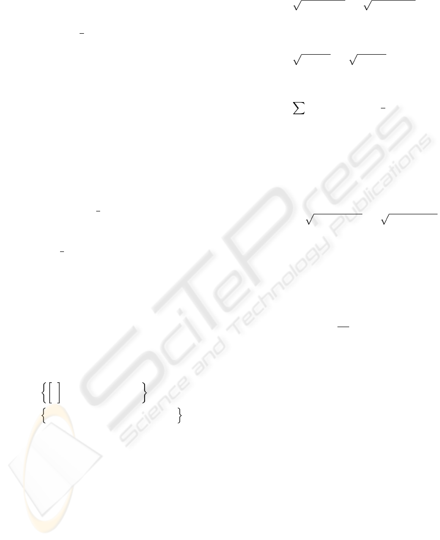
An experimental system for research of robot control

algorithms has been designed and built at The Uni-

versidad Aut

onoma de Puebla, M

exico; it is a direct-

drive robot of two degrees of freedom (see Figure 1).

The experimental robot consists of two links made

of 6061 aluminium actuated by brushless direct-drive

servo actuators from Parker Compumotor to drive the

joints without gear reduction. Advantages of this type

of direct-drive actuator includes freedom from back-

slash and signiﬁcantly lower joint friction compared

with actuators composed by gear drives. The mo-

tors used in the robot are listed in Table 1. The ser-

vos are operated in torque mode, so the motors act

as a torque source and they accept an analog volt-

age as a reference of torque signal. Position infor-

mation is obtained from incremental encoders located

on the motors. The standard backwards difference al-

gorithm applied to the joint positions measurements

was used to generate the velocity signals. The manip-

ulator workspace is a circle with a radius of 0.7 m.

A NEW FAMILY OF CONTROLLERS FOR POSITION CONTROL OF ROBOT MANIPULATORS

363

Besides position sensors and motor drivers, the robot

also includes a motion control board manufactured by

Precision MicroDynamics Inc., which is used to ob-

tain the joint positions. The control algorithm runs on

a Pentium-II (333 Mhz) host computer.

Figure 1: Experimental robot.

Table 1: Servo actuators of the experimental robot.

Link Model Torque [Nm] p/rev

1. Shoulder DM1050A 50 1,024,000

2. Elbow DM1004C 4 1,024,000

With reference to our direct-drive robot, only the

gravitational torque is required to implement the new

family of controllers (3), which is available in (Kelly,

1997):

g(q) =

38.46 sin (q

) + 1.82 sin (q

+ q

)

1.82 sin (q

+ q

)

[Nm].

The vision system consists of a camera with a focal

length λ = 0.0048 [m] and a FPG-44 frame proces-

sor board. A black disc was mounted on end-effector,

the centroid of disc was selected as the object feature

point.

The CCD camera was placed in front of the robot

and its position with respect to the robot frame Σ

was o

= [0.15, −0.55, 0.55]

[m].

5 EXPERIMENTAL RESULTS

To support our theoretical developments, this Section

presents an experimental comparison of three position

controllers on a planar robot.

We select in all controllers the desired position in

the image plane as [u

]

= [500 355]

[pix-

els] and the following initial position [u(0) v(0)]

[360 400]

[pixels] and ˙q(0) = 0 [degrees/sec]. The

friction phenomena were not modeled for compensa-

tion purposes. The evaluated controllers have been

written in C language. The sampling rate was exe-

cuted at 2.5 msec. while the visual feedback loop was

at 33 msec.

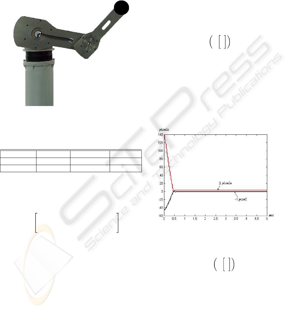
Figure 2 shows the experimental results of the con-

troller

τ = J

(q)R(θ)K

tanh

˜u

˜v

− K

tanh (Λ

+g(q). (8)

The parameters of this controller were selected

as K

= diag{23.6, 3.95} [Nm/pixels

= diag{2.0, 0.2} [Nm-sec/degrees] and

Λ = diag{0.1, 0.1}. Figure 2 depicts the time

evolution of feature error vector [˜u ˜v]

. The transient

response is fast and it was around 0.6 sec. After

transient, both components of the feature position

error tend asymptotically to a small neighborhood of

zero( 3 and -1 pixels, respectively).

Figure 2: Feature position error trajectory in the image

plane for controller (8).

The experimental results for the controller

τ = J

(q)R(θ)K

arctan

˜u

˜v

− K

arctan (Λ

+g(q)

(9)

are shown in Figure 3. The proportional and deriv-

ative gains were selected as K

= diag{15.0, 2.8}

[Nm/pixels

], K

= diag{2.0, 0.1} [Nm-

sec/degrees] respectively and Λ = diag{0.1, 0.1}.

The transient response is fast and it was around 0.5

sec. The components of the feature position error tend

asymptotically to a small neighborhood of zero ( 2

and -3 pixels, respectively).

ICINCO 2005 - ROBOTICS AND AUTOMATION

364

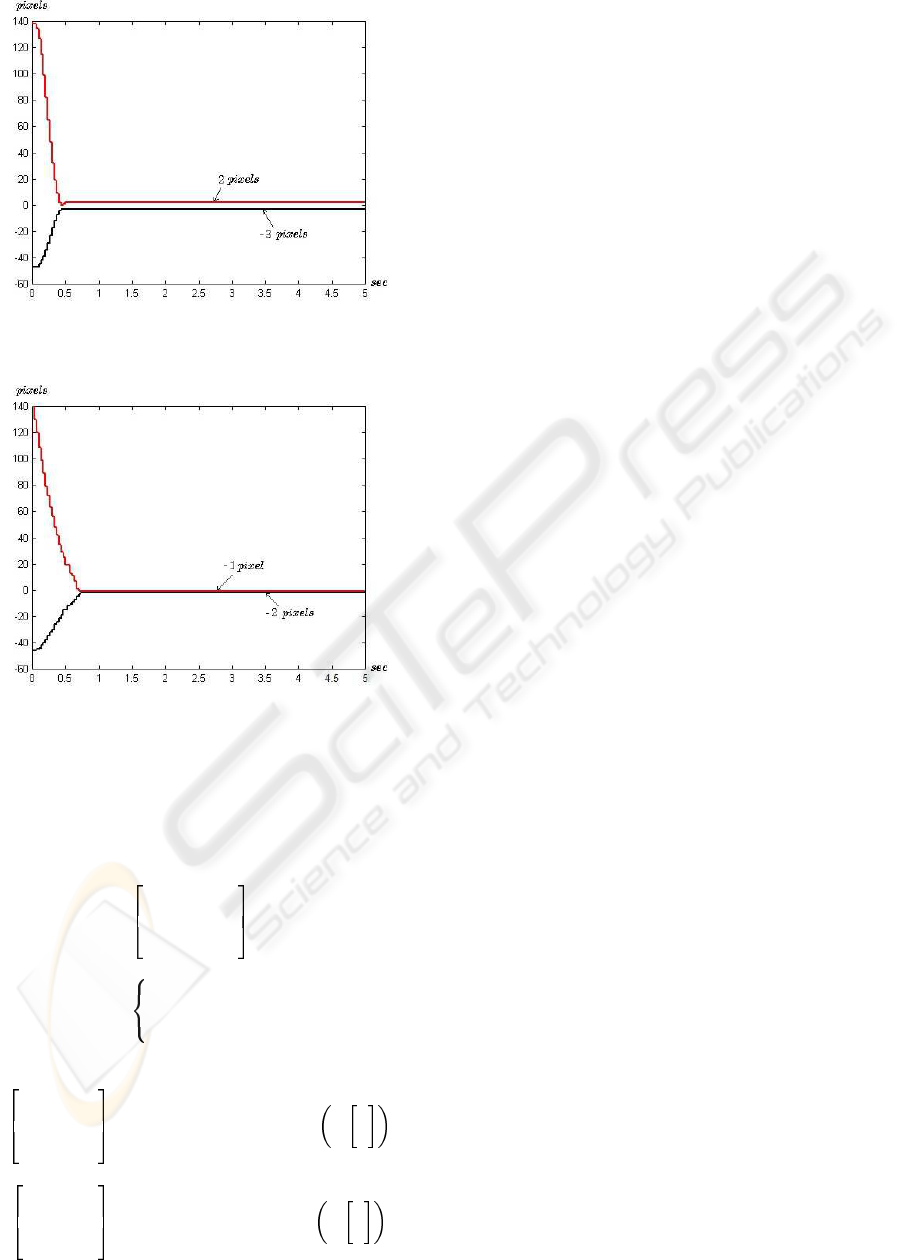
Figure 3: Feature position error trajectory in the image

plane for controller (9).

Figure 4: Feature position error trajectory in the image

plane for controller (10).

Finally the experimental results for the controller

τ = f (K

, ˜u, ˜v) − K

q + g(q) (10)

where

f (K

, ˜u, ˜v) =

, ˜u, ˜v)

, ˜u, ˜v) =

(tanh)

if |f

(sinh)

| ≥ σ

(sinh)

if |f

(sinh)

| < σ

for all i = 1, 2, ..., n and

(tanh)

= J

(q)K

R(θ) tanh Λ

˜u

˜v

(sinh)

= J

(q)K

R(θ) sinh Λ

˜u

˜v

are shown in Figure 4. The gains were se-

lected as K

= diag{25.85, 3.93} [Nm/pixels

= diag{0.17, 0.018} [Nm-sec/degrees] respec-

tively and Λ = diag{0.1, 0.1}. The transient re-

sponse was around 0.75 sec. The components of the

feature position error tend asymptotically to -1 and -2

pixels, respectively.

To compare the experimental results obtained for

the three controllers we use the L

norm (Khalil,

2002) of the feature position error. For the controller

(8) L

[˜u ˜v]

= 3.50 [pixels], then for the controller

(9) L

[˜u ˜v]

= 3.99 [pixels], ﬁnally for the controller

(10) L

[˜u ˜v]

= 2.47 [pixels]. Therefore the smallest

norm corresponds to the controller (10), then this

controller presents the best steady state performance.

6 CONCLUSIONS

This paper has introduced a new family of position

control algorithms for robot manipulators. It is sup-

ported by a rigorous stability analysis, the theoretical

results establish conditions for ensuring global reg-

ulation. The simple PD controller can be a particu-

lar member of this new scheme when its proportional

gain is a diagonal matrix. Applications for Visual Ser-

voing have been shown.

For stability purposes, the tuning procedure for the

new scheme is sufﬁcient to select a proportional gain

as diagonal matrix and derivative gain as symmetric

positive deﬁnite matrix in order to ensure global as-

ymptotic stability.

REFERENCES

A. Loria, E. Lefeber, . H. N. (2002). Global asymptotic

stability of robot manipulators with linear pid and pi

control. In SACTA.

Armstrong-Ho

elouvry, B. (1991). Control of Machines with

Friction. Kluwer Academic Publishers, Boston, 1st

edition.

B. Armstrong-Ho

elouvry, D. Neevel, . T. K. (1999). New

results in npid control: Tracking, integral control, fric-

tion compensation and experimental results. In Pro-

ceedings of the 1999 IEEE International Conference

on Robotics and Automation.

C. Canudas, B. Siciliano, . G. B. (1996). Theory of Robot

Control. Springer, Great Britain, 1st edition.

Craig, J. J. (1989). Introduction to Robotics: Mechanics and

Control. Addison–Wesley, Massachusetts, 1st edition.

F. L. Lewis, C. T. Abdallah, . D. M. D. (1993). Control

of Robot Manipulators. MacMillan Publishing Com-

pany, N.Y., 1st edition.

A NEW FAMILY OF CONTROLLERS FOR POSITION CONTROL OF ROBOT MANIPULATORS

365

J. Alvarez, R. Kelly, . I. C. (2003). Semiglobal stability of

saturated linear pid control for robot manipulators. In

Automatica.

Kelly, F. R. . R. (1997). Experimental evaluation of identi-

ﬁcation schemes on a direct drive robot. In Robotica.

Cambridge University Press.

Kelly, R. (1995). A tuning procedure for stable pid control

of robot manipulators. In Robotica. Cambridge Uni-

versity Press.

Kelly, R. (1999). Regulation of manipulators in generic task

space: An energy shaping plus damping injection ap-

proach. In IEEE Trans. on Robotics and Automation.

IEEE.

Khalil, H. K. (2002). Nonlinear Systems. Prentice–Hall,

N.J., 3rd edition.

Koditschek, D. (1984). Natural motion for robot arms. In

Proceedings of the 1984 IEEE Conf. on Decision and

Control.

L. Sciavicco, . B. S. (1996). Modeling and Control of Robot

Manipulators. The McGraw–Hill Companies, Inc.,

London, 2nd edition.

M. Takegaki, . S. A. (1981). A new feedback method for dy-

namic control of manipulators. In J. Dyn. Syst. Meas.

Control Trans. ASME.

O. Khatib, J. J. Craig, . T. L.-P. (1989). The Robotics Review

1. M.I.T. Press, Massachusetts, 1st edition.

R. Kelly, . R. C. (1996). A class of nonlinear pd–type con-

trollers for robot manipulators. In Journal of Robotic

Systems.

S. Arimoto, . F. M. (1986). Stability and robustness of pd

feedback control with gravity compensation for ro-

bot manipulator. In Robotics: Theory and Practice.

ASME winter annual meeting.

Seraji, H. (1998). A new class of nonlinear pid controllers

with robotic applications. In Journal of Robotic Sys-

tems.

V. Santiba

nez, R. Kelly, . F. R. (1998). A new set–point

controller with bounded torques for robot manipula-

tors. In IEEE Transactions on Industrial Electronics.

IEEE.

Vidyasagar, M. W. S. . M. (1989). Robot Dynamics and

Control. John Wiley & Sons, N.Y., 1st edition.

Y. Xu, J. M. Hollerbach, . D. M. (1995). A nonlinear pd

controller for force and contact transient control. In

IEEE Control Systems. IEEE.

ICINCO 2005 - ROBOTICS AND AUTOMATION

366