MUSICAL INSTRUMENT ESTIMATION FOR POLYPHONY

USING AUTOCORRELATION FUNCTIONS

Yoshiaki Tadokoro

Dept. of Information and Computer Sciences, Toyohashi University of Technology,Toyoahashi,441-8580 Japan

Koji Tanishita

Dept. of Information and Computer Sciences, Toyohashi University of Technology,Toyoahashi,441-8580 Japan

Keywords: musical instrument estimation, polyphony, autocorrelation function.

Abstract: This paper proposes a new musical instrument estimation of polyphony using autocorrelation

functions. We notice that each musical instrument has each autocorrelation function. Polyphony

can be separated into each monophony using comb filters ( ). We can obtain the

autocorrelation functions for the outputs of comb filters from the autocorrelation functions of the

monophony. By the pattern patching between the autocorrelation functions for the output signals

of the comb filters and ones calculated from monophony of each instrument, we can estimate the

musical instruments for polyphony.

zzH

−

−= 1)(

1 INTRODUCTION

Musical transcription is necessary in the musicology

field, musical retrieval and also a significant

problem in machine perception (Roads, 1985),

(Sterian and Wakefield, 2000), (Pollasri, 2002). In

the transcription, the pitch estimation is most

important and many studies have been done (Roads,

1996), (Tadokoro el al, 2001, 2002, 2003),. We also

proposed a unique method of the pitch estimation

that is based on the elimination of the pitch and its

harmonic components using the cascade or parallel

connections of the comb filters (Tadokoro el al,

2001, 2002, 2003). On the other hand, there are not

many studies for the instrument estimation(Brown

and cooke, 1994), (Abe and Ando, 1996), (Zhang,

2001), (Lee and Chun, 2002), (Krishan and

Steenivas, 2004), (Jincahita, 2004), although the

instrument estimation is also necessary in the

transcription. Most of old studies are for

monophony and based on the spectrum analysis of a

musical sound. In the recent studies, the new

technologies such as neural network, fuzzy logic

(Zhang, 2001), hidden morkov model (Lee and Chun,

2002) and independent subspace analysis (Jincahita,

2004).

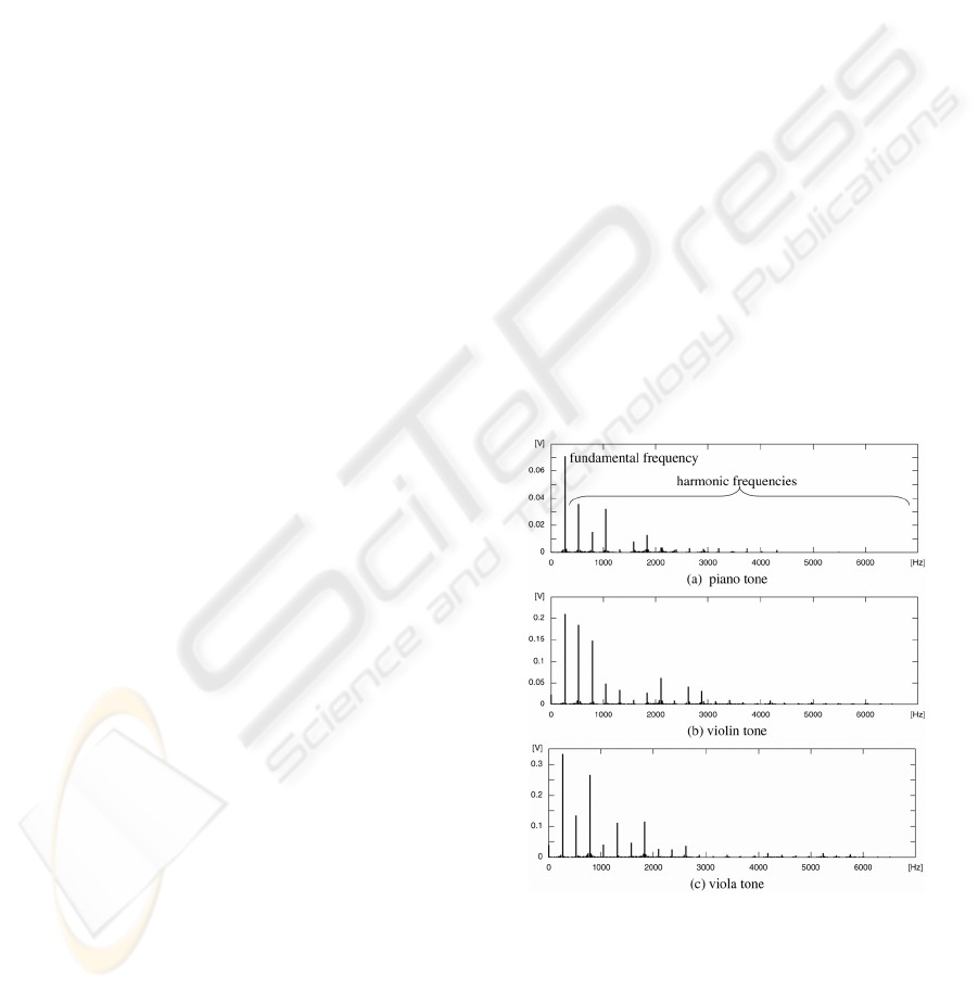
Figure 1: Spectra of tones, (a)piano, (b)violin and

(c)viola

143

Tadokoro Y. and Tanishita K. (2005).

MUSICAL INSTRUMENT ESTIMATION FOR POLYPHONY USING AUTOCORRELATION FUNCTIONS.

In Proceedings of the Second International Conference on Informatics in Control, Automation and Robotics - Signal Processing, Systems Modeling and

Control, pages 143-148

DOI: 10.5220/0001175001430148

 SciTePress

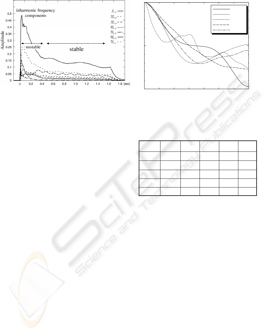
Figure 2: STFT result of piano tone

The spectrum of each musical instrument has

different frequency components as shown in Fig.1.

Therefore the instrument estimation based on the

spectrum analysis is reasonable. But there are some

problems in the instrument estimation based on the

spectrum analysis. One of them is that the spectrum

for the signal just after the instrument is played is

unstable. Figure 2 shows the result of the short-time

Fourier transform (STFT) of piano tone

C ( of

octave 4). In the range from 0.0 to 0.4 s, the each

harmonic component is changing irregularly. But,

we must estimate the instrument in a short duration

signal like about 100ms, because a sixteenth note is

125 ms at the tempo of a quarter note =120.

Another is that tones in lower octaves have lower

fundamental frequencies and to separate polyphony

into each monophony and obtain these spectra by the

FFT method, we must use a longer signal duration

necessarily. For an example, to distinguish two tones

and

#2#2 C

we must use at least a signal duration of 257 ms,

because the frequency difference between these two

tones is 3.89 Hz. That is, the method based on the

DFT must use the longer signal duration to obtain a

higher frequency resolution. On the other hand, the

method based on the parametric model such as the

linear prediction method (LPM) can calculate the

spectrum from a smaller data. Then we considered

the instrument estimation for monophony musical

sound using the LPM that could be applied to the

sounds of the shorter duration like about 50 ms

(Tadokoro et al, 2004). But, the LPM method has

the problem that it has many computations and the

prediction coefficients are sensitive to the change of

a signal waveform.

C )41.65(

Hzf

= )30.69

0244872

–1

clarinet

horn

alt–sax

viola

violin

auto–correlation R(k)

unstable

Figure 3: Autocorrelation functions of tones for

five instruments

)(kR

Table 1: Accumulated differences between the

autocorrelation functions (

) of two

instruments

)(),( kRkR

0violin

16.170viola

19.7417.190alt-sax

7.8222.7123.200horn

19.5612.5019.2524.910clarinet

violinviolaalt-saxhornclarinet

0violin

16.170viola

19.7417.190alt-sax

7.8222.7123.200horn

19.5612.5019.2524.910clarinet

violinviolaalt-saxhornclarinet

In this paper, we consider the instrument

estimation using each autocorrelation function for

each instrument. The proposed method has a smaller

computation than the LPM, because the p-order

LPM must use

autocorrelation functions and

solve the Yule-Walker equation. Furthermore, we

consider the instrument estimation for polyphony

musical sound that may be suitable to the pitch

( HzfC =

estimation method using comb filters that we

proposed.

We assume that the polyphony is composed of

two different tones of which pitches have already

estimated by the pitch estimation method. And the

input sounds are real sounds of five instruments

(clarinet, horn, alto-sax, viola and violin) and are in

octave 3 to 5. These database (RWC music database)

are made by the Real World Computing Partnership

in Japan. The sampling frequency is

The playing method is moderate but not piano or

forte.

kHzf

1.44=

ICINCO 2005 - SIGNAL PROCESSING, SYSTEMS MODELING AND CONTROL

144

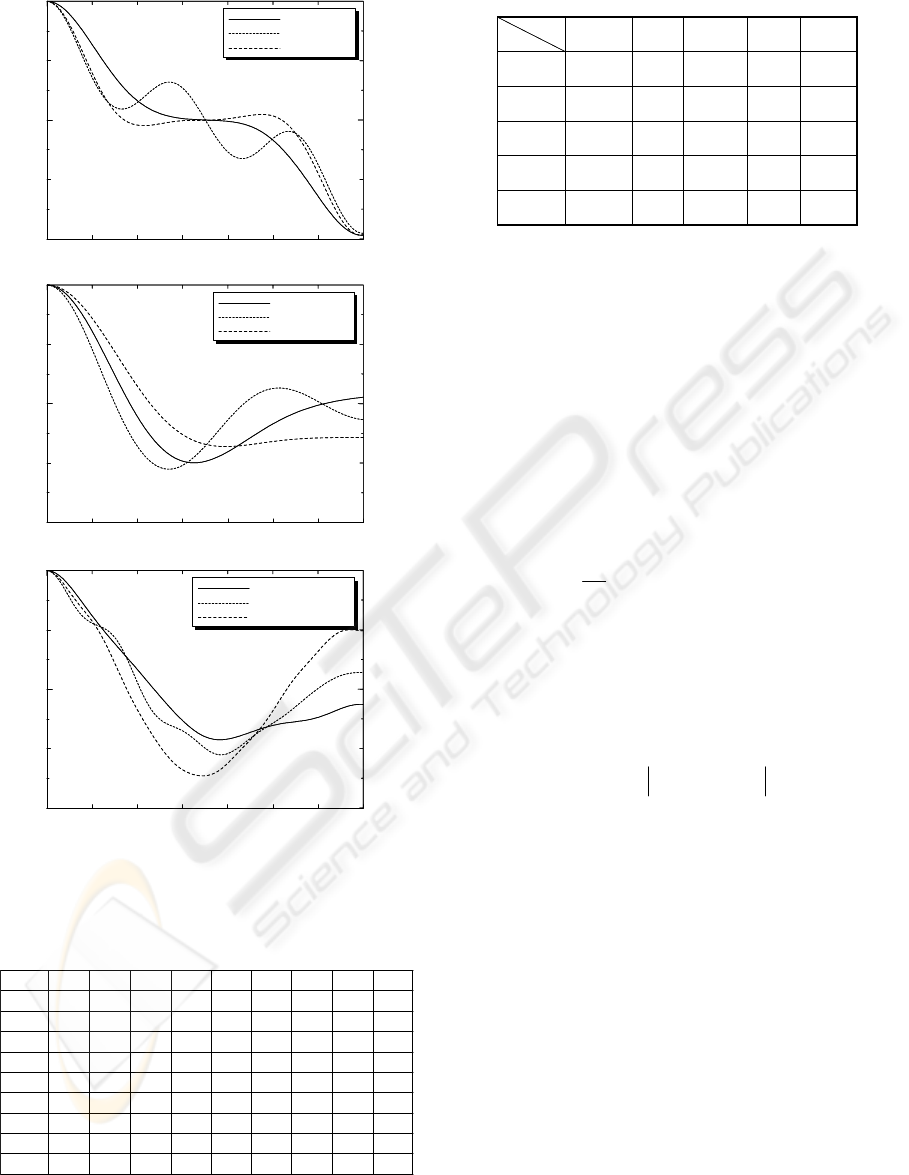
Figure 4: Autocorrelation functions of some instrument

makers

Table 2: Accumulated differences between auto-

correlations functions of some instrument makers

Table 3: Instrument estimation results for tone

982

000violin

09700viola

0010000alt-sax

0001000horn

00097clarinet

violinviolaalt-saxhornclarinet

98000violin

09700viola

0010000alt-sax

0001000horn

00097clarinet

violinviolaalt-saxhornclarinet

2 INSTRUMENT ESTIMATION

FOR MONOPHONY USING

AUTOCORRELATIO

FUNCTIONS

2.1 Autocorrelation Function of

Monophony

We calculate the autocorrelation function of a signal

by )(nx

∑

−

)()(

)(

knxnx

kR (1)

Figure 3 shows the autocorrelation functions

tones for five instruments calculated by using

)(kR

the signals of 50 ms duration in the beginning part of

the sounds. Table 1 represents the accumulated

differences of

between two instruments

showing in Eq.(2)

)(kR

∑

−=−

kRkRqpAD

)()()( (2)

From these results, we can realize that we can

estimate the instruments by the autocorrelation

functions

. )(kR

0 244872

–1

auto–correlation Rxx(k)

SELMER

YAMAHA

GEMEINHA

clarinet( )

0 244872

–1

auto–correlation Rxx(k)

SELMER

YAMAHA

GEMEINHA

clarinet( )

0 244872

–1

auto–correlation Rxx(k)

J.F.PRESSENDA

CARCASSI

FIUMEBIANCA

violin( )

0 244872

–1

auto–correlation Rxx(k)

J.F.PRESSENDA

CARCASSI

FIUMEBIANCA

violin( )

0 244872

–1

auto–correlation Rxx(k)

ALEXANDER

KNOPF

YAMAHA

horn( )

0 244872

–1

auto–correlation Rxx(k)

ALEXANDER

KNOPF

YAMAHA

horn( )

sound

est.

sound

est.

But we have one problem that the autocorrelation

functions for instruments are different depending on

the instrument makers. Figure 4 shows the

autocorrelation functions for some instruments of

some instrument makers. Table 2 represents the

accumulated differences

between these

autocorrelation functions. From these results, we

must prepare the templates for each instrument

maker.

)( qpAD −

0viol.3

34.80viol.2

23.99.70viol.1

27.212.74.10hor.3

34.111.455.538.20hor.2

13.88.4911.914.5140hor.1

3929.824.323.523.427.40clar.3

38.427.721.521.130.926.511.60clar.2

42.329.119.618.532.328.610.514.80clar.1

viol.3viol.2viol.1hor.3hor.2hor.1clar.3clar.2clar.1

0viol.3

34.80viol.2

23.99.70viol.1

27.212.74.10hor.3

34.111.455.538.20hor.2

13.88.4911.914.5140hor.1

3929.824.323.523.427.40clar.3

38.427.721.521.130.926.511.60clar.2

42.329.119.618.532.328.610.514.80clar.1

viol.3viol.2viol.1hor.3hor.2hor.1clar.3clar.2clar.1

2.2 Instrument Estimation for

Monophony

We made some experiments for the instrument

estimation under the following conditions: The

template of autocorrelation function

of each

)(

MUSICAL INSTRUMENT ESTIMATION FOR POLYPHONY USING AUTOCORRELATION FUNCTIONS

145

instrument is made at the point of 20 ms in the

beginning part of a sound, and 100 autocorrelation

functions

are made randomly in the range

from15 ms to 25 ms in the beginning part of the

sound. We made some instrument estimations for

and tones. Table 3 shows the estimation

results for

C tone. We could obtain the mean

estimation error of 0.8 % for these tones

(

)(

, CG

543

,, FCG

3 INSTRUMENT ESTIMATION

FOR POLYPHONY USING

AUTOCORRELATIO

FUNCTIONS

3.1 Separation of Polyphony Using

Comb Filter

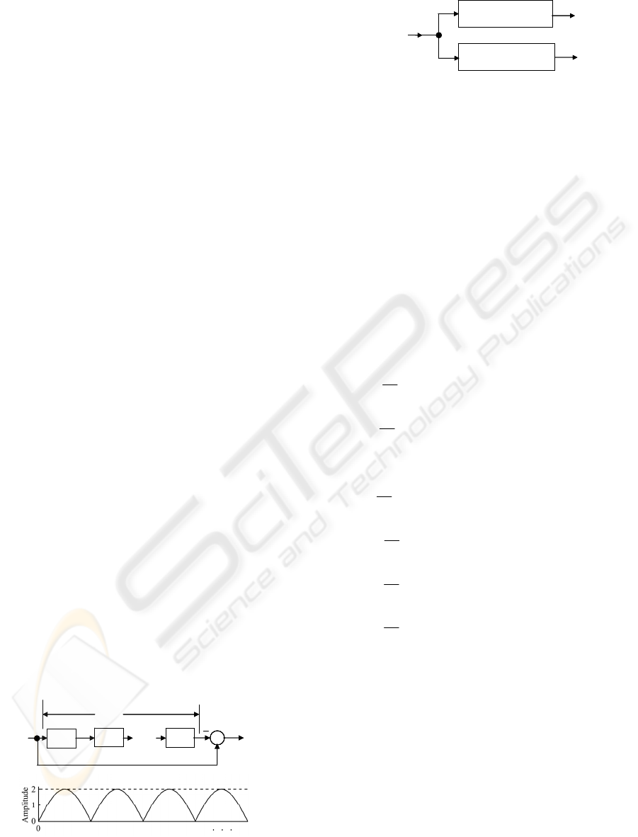
The comb filter is written by Eq.(3) and its

block diagram and the frequency characteristic are

shown in Fig.5. We can separate polyphony into each

monophony using the comb filters as shown in Fig.6.

The comb filter

can eliminate one tone

corresponding to the its period

where

one delay

)(zH

)(

spp

fNT /=

fz =

−

zzH

−

−= 1)( (3)

Because the instrument sound with pitch

composed of a fundamental frequency (pitch)

and its harmonic ones

. But the

amplitudes of

and

of each

monophony separated by the comb filters are

changed by the amplitude characteristics of the

comb filters

and , respectively.

),3,2( "=nnf

)(' nx )(' nx

)(zH

3.2 Autocorrelation Function of the

Output of a Comb Filter

(a)

(b)

Figure 5: (a) Block diagram of comb filter and (b) its

Frequency characteristic

zzH

−

−= 1)(

zzH

−

−= 1)(

)()()( nxnxnx

)(' nx

zzH

−

−= 1)(

zzH

−

−= 1)(

)()()( nxnxnx

)(' nx

Figure 6: Separation of polyphony into each monophony

The output of the comb filter is written by )(zH

)()()(

Nnxnxny

−

(4)

The autocorrelation function

of can

be calculated

by using the autocorrelation

functions for the monophony as shown in Eq.(5).

)(kR

)(ny

By using Eq.(5), we have only the same number of

autocorrelation functions for the templates as the

number of instruments per each tone. We confirmed

that the autocorrelation function of the output of the

comb filter can be calculated by Eq.(5). Figure 7

shows two autocorrelation functions, one of them is

one calculated by using the output of the comb filter

, and the other is calculated by Eq.(5) using

the autocorrelation function

for monophony

)(zH

)(kR

() () ( )

{() ( )}

{( ) ( )}

()( )

()()

2()( )( ) (5

po p p

R k ynynk

xn xn N

xn k xn k N

xnxn k

xn N xn N k

xnxn k N

xn N xn k

Rk RN k RN k

−

=−−⋅

+− +−

+−−+

−+−

−−+

=−+−−

∑

)

when two tones of the polyphony are a clarinet

and a horn

E and the comb filter

eliminates the horn E . These

autocorrelation functions are almost same. Figure 8

shows the autocorrelation functions of the output

of the comb filter H for five

instruments in the same condition as Fig.7. Table 4

)(zH

)(' nx

)(z

1−

)(nx

)(ny

)(

Nnx −

1−

)(nx

)(ny

)(

Nnx −

zzH

−

−= 1)(

zzH

−

−= 1)(

shows the values of Eq.(2) when the input sound is

composed of one tone (

) of five instruments and

a horn tone (

), and the tone is eliminated by

ICINCO 2005 - SIGNAL PROCESSING, SYSTEMS MODELING AND CONTROL

146

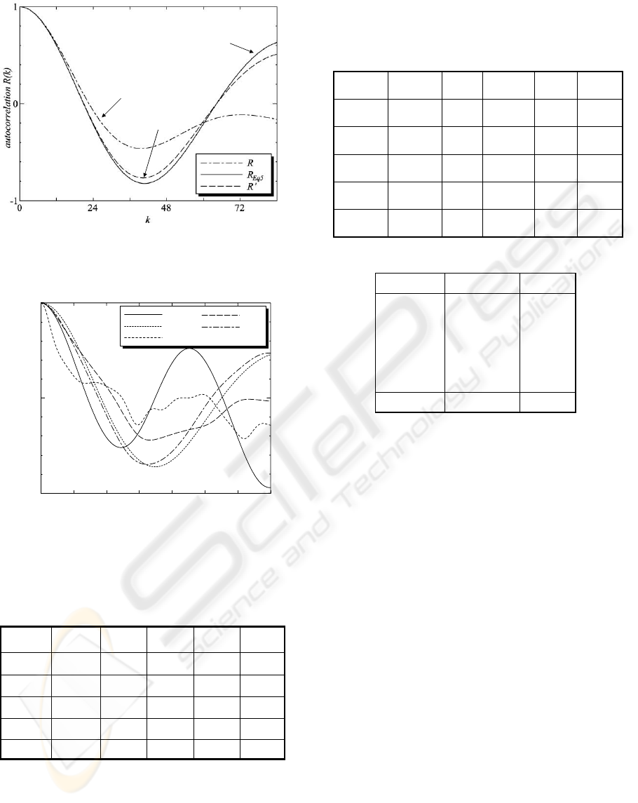
Figure 7: Comparison between autocorrelation function of

output (

) of the comb filter and one

calculated by Eq.5 using autocorrelation function

monophony (

:horn, :clarinet)

C )()(

EzH

)(kR

Figure 8: Autocorrelation functions of output of the comb

filter

for five instruments )()(

EzH

Table 4 Accumulated differences between the

autocorrelation functions ( )of two

instruments when the input sound is

and the

tone is eliminated by the comb filter

)(),( kRkR

EC +

)()(

EzH

Table 5: Instrument estimation results when the input

sound is composed of one of five instruments (

C ) and

horn (

), and the tone is eliminated by the comb

filter

( ).

)(zH

monophony

Eq.(5)

comb output

monophony

Eq.(5)

comb output

1000000violin

0100000viola

0010000alt-sax

1500850horn

0000100clarinet

violinviolaalt-saxhornclarinet

1000000violin

0100000viola

0010000alt-sax

1500850horn

0000100clarinet

violinviolaalt-saxhornclarinet

Table 6: Instrument estimation errors.

6.0mean error

4.6

12.7

2.2

4.9

6.0

clarinet

horn

alt-sax

viola

violin

error(%)sound rangeinstrument

6.0mean error

4.6

12.7

2.2

4.9

6.0

clarinet

horn

alt-sax

viola

violin

error(%)sound rangeinstrument

−

0 244872

–1

clarinet

horn

alt–sax

viola

violin

auto–correlation R(k)

the comb filter

(

). From these results, we

can realize that each autocorrelation function of the

output of the comb filter for each instrument is

different each other.

)(zH

3.3 Instrument Estimation for

Polyphony

Using the combination of five instruments, we made

the instrument estimation when two tones are

and

E . Like in the case of monophony, we

made each 100 autocorrelation functions in the

range from 15 ms to 25 ms for two outputs of the

comb filters in Fig.6. Then we

0violin

18.960viola

33.9020.200alt-sax

6.2216.7234.620horn

41.5737.2425.9044.510clarinet

violinviolaalt-saxhornclarinet

C’

0violin

18.960viola

33.9020.200alt-sax

6.2216.7234.620horn

41.5737.2425.9044.510clarinet

violinviolaalt-saxhornclarinet

C’

calculated Eq.(2) between the autocorrelation

function of the output of the comb filter and the

templates calculated by Eq.(5) for five instruments.

Table 5 shows one example of the instrument

estimation results under the same condition as Table

4. Table 6 shows the each instrument estimation

error for two tones that are made by all the

combinations of five instruments. We could obtain

the mean estimation error of 6% for five

instruments.

MUSICAL INSTRUMENT ESTIMATION FOR POLYPHONY USING AUTOCORRELATION FUNCTIONS

147

4 CONCLUSIONS

We proposed a new musical instrument estimation

of polyphony using autocorrelation functions.

Polyphony can be separated into each monophony

using the comb filters. Using the autocorrelation

functions of the outputs of the comb filters, we can

estimate the instrument by comparing with the

autocorrelation functions of the templates that can be

calculated from the autocorrelation functions of

monophony. We could obtain the mean estimation

error of 6% for five instruments.

As a future work, we’d like to reduce the number

of templates considering the analogous

autocorrelation functions of neighbour tones.

REFERENCES

M.Abe and S.Ando, “Application of loudness/

pitch/timbre decomposition operators to auditory scene

analysis,” Proc. of ICASP.pp.2646-2649, 1996.

G.J.Brown and M.Cooke, “Perceptual grouping of musical

sounds: a computational model,” Journal of New

Music Research, vol.23, no.2 pp.107-132, 1994.

P.Jincahita, “Polyphonic instrument identification suing

independent subspace analysis,” IEEE Int. Conf. on

Multimedia and Xpo (ICME), vol.2, pp.1211-1214,

2004

A.G.Krishna, and T.V.Sreenivas, “Music instrument

recognition: From isolated notes to solo phrases,” Proc.

Of ICASSP, pp.IV265-268, 2004

J.Lee and J.Chun, “Musical instrument recognition using

hidden morkov model,” Conference record of the

Asilomar Conference on Signals, Systems and

Computers, vol.1, pp.196-199, 2002

E.Pollastri, ”A pitch tracking system dedicated to process

singing voice for musical retrieval,” Proc. of IEEE Int.

Conf. on Multimedia and Xpo (ICME) , 2002.

C.Roads, ”Research in music and artificial intelligence,”

ACM computing Survey, vol.17, no.2, pp.163-190,

1985.

C.Roads, ”The Computer Music Tutorial,” MIT Press,

1996.

A.Sterian and G.H.Wakefield, ”Music transcription

systems: from sound to symbol,” Proc. of AAAI-2000

workshop on artificial intelligence and music, July

2000.

Y.Tadokoro and T.Miwa, ”Musical pitch and instrument

estimation of polyphony using comb filters for

transcription,” 4

World Multiconference on Circuits,

Systems, Communications and Computers

(CSCC2000), Advance in Physics, Electronics and

Signal Processing Applications, pp.315-319, 2000.

Y.Tadokoro and M.Yamaguchi, “Pitch detection of duet

song using double comb filters,” Proc. of ECCTD’01,

I, pp.57-60, 2001.

Y.Tadokoro, W.Matsumoto and M.Yamaguchi, “Pitch

detection of musical sounds using adaptive comb filters

controlled by time delay,” ICME2002, P03, 2002.

Y.Tadokoro, T.Morita and M.Yamaguchi, “Pitch detection

of musical sounds noticing minimum output of parallel

connected comb filters, “ IEEE TENCON2003, tencon-

072, 2003.

Y.Tadokoro, K.Tanishita and M.Yamaguchi, ”Musical

instrument estimation using linear prediction method,”

Proceedings of the 11

International Workshop on

Systems, Signals and Image Processing(IWSSIP’04),

pp.2077-210, September 13-15, 2004.

T.Zhang, ”Instrument classification in polyphonic music

based on timbre analysis,” Proc. of SPIE, vol.4519,

pp.136-147, 2001

ICINCO 2005 - SIGNAL PROCESSING, SYSTEMS MODELING AND CONTROL

148