
OPTIMIZATION IN RAILWAY SCHEDULING
M.A. Salido
1
, M. Abril
1
, F. Barber
1
, L. Ingolotti
1
,A.Lova
2
, P. Tormos
2
1
Departamento de Sistemas Inform
´
aticos y Computaci
´
on
2
Departamento de Estad
´
ıstica e I.O y Calidad
Universidad Polit
´
ecnica de Valencia
Keywords:
optimization, constraint optimization, railway scheduling problem.
Abstract:
Train scheduling has been a significant issue in the railway industry. Over the last few years, numerous ap-
proaches and tools have been developed to aid in the management of railway infrastructure. In this paper, we
describe some techniques, which was developed in a project in collaboration with the Spanish Railway In-
fractructure Manager (ADIF). We formulate train scheduling as constraint optimization problems and present
two filtering techniques for these problem types. These filtering techniques are developed to speed up and
direct the search towards suboptimal solutions in periodic train scheduling problems. The feasibility of our
problem-oriented techniques are confirmed with experimentation using real-life data. The results show that
these techniques enables MIP solvers such as LINGO and ILOG Concert Technology (CPLEX
c
) to terminate
earlier with good solutions.
1 INTRODUCTION
Railway transportation has played a major role in the
economic development of the last two centuries. It
represented a major improvement in land transport
technology and has obviously introduced important
changes in the movement of freight and passengers.
Over the last few years, railway traffic has increased
considerably, which has created the need to optimize
the use of railway infrastructures. This is, however,
a very difficult task. Nevertheless, numerous ap-
proaches and tools have been developed to aid in the
management of railway infrastructure. These systems
provide advanced graphical interfaces, but they still
lack of benefits for automatic planning of efficient
and robust scheduling. Thanks to developments in
computer science and advances in the fields of opti-
mization and intelligent resource management, rail-
way managers can optimize the use of available in-
frastructures, obtain more robust timetables and ob-
tain useful conclusions about capacity of their topol-
ogy.
We describe some results of a long-term collab-
oration between our research group and the Span-
1
This work has been partially supported by the grant
TIN2004-06354-C02- 01 (MEC, Spain - FEDER) and
GV04B/516 (Generalitat Valenciana, Spain).
ish Railway Infractructure Manager (ADIF) (Mom,
2005). The aim of the project is to offer assistance in
the planning of train scheduling to obtain conclusions
about the maximum capacity of the network, to iden-
tify bottlenecks, to provide support in the resolution
of incidents, etc. Besides the mathematical processes,
a high level of interaction with railway experts is re-
quired to be able to take advantage of their experi-
ence.
In this paper, we propose two problem-oriented fil-
tering techniques for solving periodic train schedul-
ing. The train scheduling problem has received con-
siderable attention in the literature: (Szpigel, 1972) is
the first to propose a branch and bound algorithm for
train scheduling; (Higgins, 1997) define local search,
tabu search, genetic and hybrid heuristics; (Cai, 1994)
illustrate a constructive greedy heuristic. Periodic
timetables for railway networks is usually modeled
by Periodic Event Scheduling Problem (PESP) (Ser-
afini, 1989). It is known that the PESP is NP-hard
(Serafini, 1989). Approaches to solve PESP instances
cover backtracking strategies in a branch-and-bound
context (Serafini, 1989), genetic algorithms (Nachti-
gall, 1996), and some classes of cutting planes (Odijk,
1994). Furthermore, several European companies are
also working on similar systems. These systems in-
clude complex stations, rescheduling due to incidents
188
A. Salido M., Abril M., Barber F., Ingolotti L., Lova A. and Tormos P. (2005).
OPTIMIZATION IN RAILWAY SCHEDULING.
In Proceedings of the Second International Conference on Informatics in Control, Automation and Robotics, pages 188-195
DOI: 10.5220/0001176101880195
Copyright
c
SciTePress

(Chiu et al., 2002), rail network capacities (Kaas,
1998), etc. These are complex problems for which
work in network topology and heuristic-dependent
models can offer appropriate solutions.
The problem formulation is (traditionally) trans-
lated into a formal mathematical model to be solved
for optimality by means of mixed integer program-
ming (MIP) techniques. However, in realtime-
environments, with hundred of trains, in different di-
rections, along paths of dozens of stations, with con-
straints about departure and arrival times, generate
thousands of inequalities and a high number of vari-
ables take only integer values. As is well known,
this type of model is far more difficult to solve than
linear programming models. In our framework, the
formal mathematical model is simplified by filtering
techniques in order to speed up the efficiency of well-
known solvers.
2 PRELIMINARIES
2.1 Terminology
A running map contains information regarding rail-
way topology (stations, tracks, distances between sta-
tions, traffic control features, etc.) and the schedules
of the trains that use this topology (arrival and depar-
ture times of trains at each station, frequency, stops,
junctions, crossings, etc,). A sample of a running map
is shown in Figure 1, where several train crossings can
be observed. On the left side of Figure 1, the names of
the stations are presented and the vertical line repre-
sents the number of tracks between stations (one-way
or two-way). The objective of our system is to obtain
a correct and optimized running map taking into ac-
count: (i) traffic rules, (ii) user requirements and (iii)
the railway infrastructure topology.
A railway network is basically composed of sta-
tions and one-way or two-way tracks. A dependency
can be: Station: is a place for trains to park, stop
or pass through. Each station is associated with a
unique station identifier. There are two or more tracks
in a station where crossings or overtaking can be
performed; Halt: ia a place for trains to stop, pass
through, but not park. Each halt is associated with a
unique halt identifier.
In Figure 1, horizontal dotted lines represent halts,
while continuous lines represent stations. On a rail
network, the user needs to schedule the paths of n
trains going in one direction and m trains going in the
opposite direction. These trains are of a given type
and a scheduling frequency is required.
The type of trains to be scheduled determines the
time assigned for travel between two locations on the
path. The path selected by the user for a train trip
determines which stations are used and the stop time
required at each station for commercial purposes. In
order to perform crossing in a section with a one-way
track, one of the trains should wait in a station. This is
called a technical stop. One of the trains is detoured
from the main track so that the other train can cross
or continue.
2.2 Problem Statement
There are three groups of scheduling rules in our rail-
way system: traffic rules, user requirements rules and
topological rules. A valid running map must satisfy
and optimize the above rules. These scheduling rules
can be modeled using the following constraints:
1. Traffic rules guarantee crossing and overtaking
operations. The main constraints to take into ac-
count are:
• Crossing constraint: Any two trains going in
opposite directions must not simultaneously use
the same one-way track.
The crossing of two trains can be performed only
on two-way tracks and at stations, where one of
the two trains has been detoured from the main
track. Several crossings are shown in Figure 1.
• Expedition time constraint. There exists a given
time to put a detoured train back on the main
track and exit from a station.
• Reception time constraint. There exists a given
time to detour a train from the main track so that
crossing or overtaking can be performed.
2. User Requirements: The main constraints due to
user requirements are:
• Type and Number of trains going in each direc-
tion to be scheduled.
• Path of trains: Locations used and Stop time for
commercial purposes in each direction.
• Scheduling frequency. The frequency require-
ments of the departure of trains in both direc-
tions. This constraint is very restrictive because,
when crossing are performed, trains must wait
for a certain time interval at stations. This in-
terval must be propagated to all trains going in
the same direction in order to maintain the es-
tablished scheduling frequency. The user can
require a fixed frequency, a frequency within
a minimum and maximum interval, or multiple
frequencies.
• Departure interval for the departure of the first
trains going in both the up and down directions.
• Maximum slack. This is the maximum percent-
age δ that a train may delay with respect to the
minimum journey time.
OPTIMIZATION IN RAILWAY SCHEDULING
189

INFORM
Stations
Halts
Time
Paths
Tracks
Figure 1: A sample of a running map
3. Topological railway infrastructure and type of
trains to be scheduled give rise other constraints to
be taken into account. Some of them are:
• Number of tracks in stations (to perform techni-
cal and/or commercial operations) and the num-
ber of tracks between two locations (one-way or
two-way). No crossing or overtaking is allowed
on a one-way track,
• Time constraints, between each two contiguous
stations,
• Added Station time constraints for technical
and/or commercial purposes.
In accordance with user requirements, the system
should obtain the best solution available so that all
the above constraints are satisfied. Several criteria can
exist to qualify the optimality of solutions: minimize
duration and/or number of technical stops, minimize
the total time of train trips (span) of the total schedule,
giving priority to certain trains, etc.
2.3 The Formal Mathematical Model
Our formal mathematical model can be described as a
constraint optimization problem, where the main ob-
jective function is to minimize the journey time of all
trains. Variables are frequencies, arrival and departure
times of trains at stations and binary auxiliary vari-
ables generated for modelling disjunctive constraints.
Constraints are composed by user requirements, traf-
fic rules, and topological constraints. These con-
straints are composed by the parameters defined by
user interfaces and database accesses.
The formal mathematical model is presented in Ta-
ble 1. Let’s suppose a railway network with r sta-
tions, n trains running in the down direction, and m
trains running in the up direction. We assume that
two connected stations have only one line connect-
ing them. T
i
A
k
represents that train i arrives at sta-
tion k; T
i
D
k
means that train i departs from station k;
Timei
k−(k+1)
is the journey time of train i to travel
from station k to k +1; TSi
k
and CSi
k
represent
the technical and commercial stop times of train i in
station k, respectively; and ET
i
and RT
i
are the ex-
pedition and reception time of train i, respectively.
The main complexity of the problem derives in
solving the MIP problem due to the binary (integer)
variables. These integer variables are generated to
manage disjunctive constraints. If we are able to as-
sign values to these integer variables, the linearized
problem can be solved more efficiently. Therefore,
the main goal of our filtering techniques is to find val-
ues for these integer variables. This assignment will
be carried out by means of local search and railway
topological knowledge.
3 FILTERING TECHNIQUES
Given the formal mathematical model presented in
Table 1, the problem turns into a MIP problem, in
which thousands of inequalities have to be satisfied
ICINCO 2005 - INTELLIGENT CONTROL SYSTEMS AND OPTIMIZATION
190
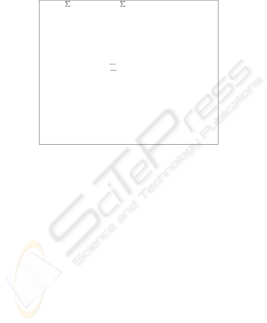
Table 1: Formal Mathematical Model of the railway scheduling problem.
(1) Min
i=n
i=1
(T
i
A
r
− T
i
D
1
)+
i=m
j=1
(T
j
A
1
− T
j
D
r
);
Subject To
/frequency constraint ∀i =1..n, ∀k =1..r
(2) T
i+1
D
k
− T
i
D
k
= F r equency;
/Time Constrains ∀i =1..n, ∀k =1..r
(3.1) T
i
A
k+1
− T
i
D
k
= Timei
k−(k+1)
;
(3.2) T
j
A
k
− T
i
D
k+1
= Timei
k−(k+1)
;
/Stations Time Constrains ∀i =1..n, ∀k =1..r
(4) T
i
D
k
− T
i
A
k
− TSi
k
= CSi
k
;
/Constrains to limit journey time ∀i =1..n, ∀j =1..m
(5.1) T
i
A
r
− T
i
D
1
≤ (1 +
δ
100
) ∗ Timei
1−r
;
(5.2) T
j
A
1
− T
j
D
r
≤ (1 +
δ
100
) ∗ Timej
r−1
;
/Crossing Constrains ∀i =1..n, ∀j =1..m, ∀k =1..r
(6.1) T
j
A
k
− T
i
D
k
<= 86400 ∗ Y
i−j;k−(k+1)
;
(6.2) T
i
A
k+1
− T
j
D
k+1
<= 86400 ∗ (1 − Y
i,j,k
);
/Expedition time constrains ∀i =1..n, ∀j =1..m, ∀k =1..r
(7.1) T
j
A
k
− T
i
D
k
− 86400 ∗ (X
i,j
− Y
i,j,k
+ Y
i,j,k+1
− 1) + ET
i
<=0;
(7.2) T
i
A
k
− T
j
D
k
− 86400 ∗ (X
i,j
− Y
i,j,k
+ Y
i,j,k+1
− 2) + ET
j
<=0;
/Reception time constrains ∀i =1..n, ∀j =1..m, ∀k =1..r
(8.1) T
i
A
k
− T
j
A
k
− 86400 ∗ (X
i,j
− Y
i,j,k
+ Y
i,j,k+1
− 1) + RT
i
<=0;
(8.2) T
j
A
k
− T
i
A
k
− 86400 ∗ (X
i,j
− Y
i,j,k
+ Y
i,j,k+1
− 2) + RT
j
<=0;
/Binary Constraints
X
i−j
; ∀i =1..n, ∀j =1..m
Y
i−j;k−(k+1)
; ∀i =1..n, ∀j =1..m, ∀k =1..r
and a high number of variables only take integer val-
ues. As is well known, this type of model is far more
difficult to solve than linear programming models.
Our filtering techniques work on the binary variables.
These variables are grouped into two sets:
• Variables Y
s. A variable Y
i,j,k
determines the
track between station k and station k +1in which
train i crosses with train j.IfY
i,j,h−1
=1for
h ≤ k and Y
i,j,p
=0for p ≥ k then, the crossing
between train i and train j is carried out in station
k.
• Variables X
s. A variable X
i,j
determines which
train (i or j) arrives earlier to the crossing station.
If X
i,j
=0train i arrives at the crossing station
first and train j arrives at the same station later.
3.1 Filtering Technique 1
This technique carries out a filtering over the set of
constraints from the formal mathematical model pre-
sented in Table 1. Many constraints of type (6) (7) and
(8) can be removed according to their departure times
and maximum slacks. If a train going in the down di-
rection arrives at the destination before a train going
in the up direction departs, then both trains will not
cross each other. Thus, a huge number of constraints
and integer variables we can eliminated. The original
problem maintains n ∗ m ∗ r integer variables (Y
s)
and n ∗ m integer variables (X
s). A railway net-
work with 100 stations and 100 trains going in each
direction generates 1.01x10
6
integer variables. This
technique may significantly reduce the problem size
with a reasonable maximum slack (α ≈ 20%) (given
by railway operator).
Theorem 2. Filtering technique 1 is sound and
complete.
Proof. Soundness. Filtering technique 1 is sound
due to the fact that the set of solutions given by Ta-
ble 1 subsumes the set of solutions obtained by filter-
ing technique 1. This is because it has removed a set
of binary variables and the constraints in which these
variables are involved.
Completeness. Filtering technique 1 does not re-
move any solution. Thus, this technique will find the
same solution as the one obtained by Table 1. Con-
straints of type (5) make the set the of removed con-
straints redundant by filtering technique 1. By contra-
diction, we assume that there is a solution that filter-
ing technique 1 does not find. Without loss of gener-
ality, we assume a maximum slack of 20%. We can
distinguish two different cases. (1) The lost solution
falls into the maximum slack. This os a contradiction
because, under this threshold, the restricted problem
is the same as Table 1. (2) The lost solution falls out-
side the maximum slack. This solution is not valid
because it does not satisfy constraints (5.1) and (5.2).
Therefore, filtering technique 1 does not lose any so-
lution.
OPTIMIZATION IN RAILWAY SCHEDULING
191

3.2 Filtering technique 2
Filtering technique 2 is a metaheuristic based on Fil-
tering technique 1. This technique carries out a
guided local search over the binary variables. Once
many integer variables have been removed by filter-
ing technique 1, a new filtering process on the re-
duced problem can eliminate other integer variables
by means of a guided local search. Instead of assign-
ing a random station as a crossing station between
two opposite trains, filtering technique 2 performs a
linearized execution where the integer variables have
been transformed into continues ones. Thus, the
crossing between two trains may not be assigned in
stations but on a track between two stations. This will
be the initial point to start the search to find the sta-
tion where the crossing will finally be performed. The
search of each crossing between two opposite trains is
bounded by 2n +1contiguous tracks. This interval
is composed by n tracks located before the obtained
crossing and n tracks located after the crossing. In
this way, the resultant subproblem can be seen as a
combinatorial problem, where all combinations must
be performed for guarantee the best possible solution.
If the problem has a solution, filtering technique 2
studies the arrival order to the crossing station such
as the objective function is minimized. Otherwise,
the interval is increased (n ++) and the MIP prob-
lem is again solved. This technique is useful in any-
time environment due to a solution can be found, but
filtering technique 2 tries to find a better solution in
the remaining time. To this end, each combination is
labelled with the solution obtained and the filtering
technique searches neighbor combination in order to
improve the objective function.
Table 2: Pseudo-code of filtering technique 2.
Filtering technique 2
{ /*Limit the stations where two trains can be crossed,
i.e., the number of integer variables*/
DeterminePossibleCrossing();
LinearSolution=SolveLinearProblem();
Crossings=DetectCrossings(LinearSolution);
n=0;
while(Not Solution) {
Solution=SearchCrossCombination(window,Crossings);
n++;
}
if (Solution)
FinalSolution=SolveCrossingOrder(Solution);
}
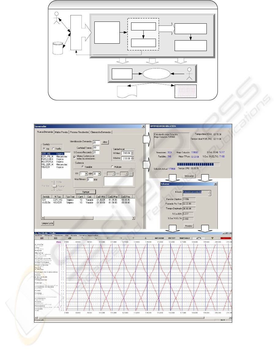
4 GENERAL SYSTEM
ARCHITECTURE
The general outline of our system is presented in Fig-
ure 2. It shows several steps, some of which require
the direct interaction with the human user to insert
requirement parameters, parameterize the constraint
solver for optimization, or modify a given schedule.
First of all, the user should require the parameters of
the railway network and the train type from the central
database (Figure 2).
This database stores the set of locations, lines,
tracks, trains, etc. Normally, this information does not
change, but authorized users may desire to change this
information. With the data acquired from the data-
base, the system generates the formal mathematical
model.
According to the quality of the required solution
and the problem size, a filtering technique will be ex-
ecuted by one of the following ways:
1. Complete: The process is performed taking into ac-
count the entire problem. This decision is carried
out when the number of trains and stations is low
or the running time is not a important. In this case,
filtering technique 1 will be selected.
2. Incremental: The process performs an incremental
coordination of trains. It can be useful in anytime
systems, where the number of trains and stations
is not very high. In this case, filtering technique
1 and 2 are appropriate due to the fact that as the
number of combinations are checked, the quality
of the solution is better.
Once the problem has been filtered, the optimiza-
tion process will be executed for obtaining an opti-
mal solution of the simplified problem. To this end,
CPLEX and LINGO are executed for obtaining the
optimal solution.
However, the system can also automatically recom-
mend or select the appropriate choice depending on
main parameters and the complexity of the problem.
If the mathematical model is not feasible, the user
must modify the parameters, mainly the most restric-
tive ones. If the running map is consistent, the graphic
interface plots the scheduling. Afterwards, the user
can graphically interact with the scheduling to mod-
ify the arrival or departure times. Each interaction
is automatically checked by the constraint checker in
order to guarantee the consistency of changes. The
user can finally print out the scheduling, to obtain re-
ports with the arrival and departure times of each train
in each location, or graphically observe the complete
scheduling topology.
ICINCO 2005 - INTELLIGENT CONTROL SYSTEMS AND OPTIMIZATION
192
Data
Base
Starting Interface
Formal
Mathematical
Model
INFORM
Plotter
Constraint
Checker
Timetabling
Graphic Interface
General Scheme
Optimization
Process
Filtering
Technique 1
Filtering
Technique 2
Running Map
Data
Figure 2: General scheme of our tool.
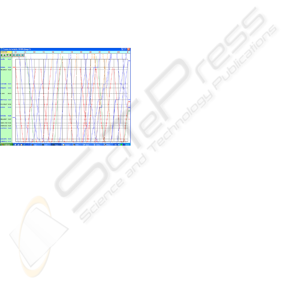
Figure 3: System Interface solving and plotting instance <10,40,90>.
4.1 A Constraint-based System for
Automatic Railway Scheduling
Our techniques described here can be extended to
general problems such as: inserting a new train or
several new trains in an already compatible running
map and optimizing running maps. In this case, new
constraints must be taken into account such as clos-
ing constraints, exclusiveness constraints, precedence
constraints, etc. Figure 4 shows an example of a high
OPTIMIZATION IN RAILWAY SCHEDULING
193
loaded running map with the proposed system.
Out tool provides several benefits for automatic
railway infrastructure scheduling.
• It is flexible and friendly. It can be easily inte-
grated into already existing data-bases and other
computer-aided tools for railway management.
• It automatically obtains optimized and well-formed
running maps (timetables).
• It can validate complex timetables by automatically
performing all the consistency checks required for
well-formed timetables.
• It can validate and perform capacity analyses.
• It can reschedule running maps according to inci-
dences and delays in on-line, traffic management.
Figure 4: Example of a high loaded running map.
5 EVALUATION
The application and performance of this system de-
pends on several factors: Railway topology (loca-
tions, distances, tracks, etc.), number and type of
trains (speeds, starting and stopping times, etc.), fre-
quency ranges, initial departure interval times, etc.
In this section, we compare the performance of
our filtering techniques using some well-known con-
straint optimization problem solvers, CPLEX and
LINGO, because they are the most appropriate tools
for solving these types of problems.
This empirical evaluation was carried out on a real
railway infrastructure that joins two important Span-
ish cities (”La Coru
˜
na” and ”Vigo”). The journey be-
tween these two cities is currently divided by 40 de-
pendencies between stations (23) and halts (17).
In our empirical evaluation, each set of instances
was defined by the 3-tuple < n,s,f >, where n was
the number of trains in each direction, s the number of
stations/halts and f the frequency. The problems were
generated by modifying these parameters. Thus, each
of the tables shown sets two of the parameters and
varies the other one in order to evaluate the algorithm
performance when this parameter increases. It must
be taken into account that running time of the form
”>xh.” represents that the problem did not finish in
x hours and the best solution found up to date is pre-
sented in the journey time column. All running times
in Table 3 represent the running times of the filtering
techniques plus the running times of the optimization
techniques (CPLEX or LINGO).
In Table 3 (a), we present the running time and the
journey time in problems where the number of trains
was increased from 5 to 75, and the number of sta-
tions/halts and the frequency were set at 40 and 90,
respectively: <n,40, 90 >. The results show as the
number of trains increased the running time of Filter-
ing technique 1 and 2 was worse. Filtering technique
1 obtained the optimal solution for 5,10,15 and 20
trains. However for 50 and 75 trains, Filtering tech-
nique 1 was aborted in 5 hours while Filtering tech-
nique 2 finished although with worse solutions. Fig-
ure 3 shows the system interface executing our Fil-
tering technique 2 with the instance < 10, 40, 90 >.
The first window shows the user parameters, the sec-
ond window presents the best solution obtained at that
point, the third window presents data about the best
solution found, and finally the last window shows the
obtained running map.
Table 3 (b) shows the running time and the jour-
ney time in problems where the number of stations
was increased from 10 to 60, and the number of trains
and the frequency were set at 10 and 90, respectively:
< 10,s,90 >. In this case, only stations were in-
cluded to analyze the behavior of the techniques. It
can be observed that Filtering technique 2 was bet-
ter than Filtering technique 1 obtaining optimal solu-
tions for 10 and 20 stations in lower time. Eve for
30 stations Filtering technique 2 had better behaviour
than Filtering technique 1 (complete algorithm). It
is important to note the difference between the in-
stance < 10, 40, 90 > of the Table 3 (a) and the in-
stance < 10, 40, 90 >
in Table 3 (b). They repre-
sent the same instance; however in Table 3 (b) we
only used stations (no halts), so the number of pos-
sible crossing between trains was much larger (more
integer variables). This item reduced the journey time
from 2:20:19 to 2:20:10, using Filtering technique 1
and from 2:26:04 to 2:23:36, using CPLEX and Filter-
ing technique 2. Nevertheless, the running time also
increased from 337” to 2131 in Filtering technique 1
and from 8” to 56” in Filtering technique 2, due to the
number of integer variables was much larger.
In Table 3 (c), we present the running time and the
journey time in problems where the frequency was de-
creased from 140 to 60 and the number of trains and
the number of stations were set at 20 and 40, respec-
ICINCO 2005 - INTELLIGENT CONTROL SYSTEMS AND OPTIMIZATION
194
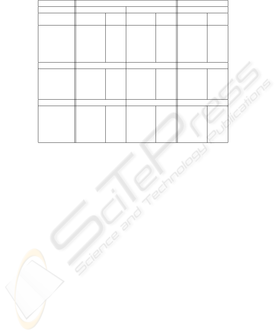
Table 3: Running time and journey time in different problem instances.
CPLEX LINGO
(a) <n,40,90> Filtering technique 1 Filtering technique 2 Filtering technique 2
Trains running time journey running time journey running time journey
time time time
5 6” 2:19:48 4” 2:29:33 6” 2:30:54
10 337” 2:20:19 8” 2:22:08 12” 2:31:37
15 601” 2:20:29 12” 2:26:18 19” 2:31:51
20 1065” 2:20:34 16” 2:26:25 25” 2:31:58
50 > 5h. 2:20:43 43” 2:31:09 1098” 2:32:11
75 > 5h. 2:22:04 > 1h. 2:32:14 1590” 2:32:14
(b) <10,s,90>
10 3” 0:25:06 2” 0:25:06 4” 0:25:06
20 303” 1:04:11 5” 1:04:11 8” 1:04:11
30 > 1h. 1:45:38 6” 1:45:08 14” 1:45:38
40 2131” 2:20:10 56” 2:23:36 21” 2:24:36
60 > 3h. 3:33:15 217” 3:39:30 180” 3:40:30
(c) <20,40,f>
140 15” 2:16:19 15” 2:20:18 24” 2:16:19
120 156” 2:16:17 14” 2:16:17 23” 2:18:47
100 > 5h. 2:22:55 15” 2:23:10 28” 2:22:55
90 1065” 2:20:34 15” 2:26:25 28” 2:31:58
75 > 1h. 2:29:18 > 1h. - 25” 2:24:16
60 > 1h. 2:21:23 > 1h. - > 1h. -
tively: < 20, 40,f >. As the frequency decreased,
the process solving become harder. The quality of
the solutions depends mainly of the network topology.
For this reason, Filtering technique 2 obtained the
same solutions than Filtering technique 1 but lower
running times with frequencies of 140, 120 and 100
minutes. It can be observed that depending on the
problem topology, one technique may be better than
the others. Therefore, it may be useful for the system
to automatically select the appropriate technique.
6 CONCLUSIONS
We have reported the design and development of two
filtering techniques for solving periodic train schedul-
ing, which is a project in collaboration with the Na-
tional Network of Spanish Railways (RENFE), Spain.
We have formulated the train scheduling as constraint
optimization problems. Two filtering techniques are
developed to speed up and direct the search towards
sub-optimal solutions. The feasibility of our algo-
rithms are confirmed with experimentation using real-
life data. These techniques have been inserted into the
system to solve periodic timetables more efficiently.
This system is already integrated and assist to railway
managers in optimizing the use of railway infrastruc-
tures and will also help them in the resolution of com-
plex scheduling problems. It supposes the application
of methodologies of Artificial Intelligence in a prob-
lem of great scientific and commercial interest.
REFERENCES
Cai, X., G. C. (1994). A fast heuristic for the train schedul-
ing problem. Computers and Operations Research 21,
pages 499–510.
Chiu, C., Chou, C., Lee, J., Leung, H., and Leung, Y.
(2002). A constraint-based interactive train reschedul-
ing tool. Constraints, 7:167–198.
Higgins, A., K. E. F. L. (1997). Heuristic techniques for
single line train scheduling. Journal of Heuristics 3,
pages 43–62.
Kaas, A. (1998). Methods to calculate capacity of railways.
Ph. Dissertation.
Mom (2005). An automated decision sup-
port tool for railway traffic management.
http://www.dsic.upv.es/users/ia/gps/MOM/.
Nachtigall, L., V. S. (1996). A genetic algorithm approach
to periodic railway synchronization. Computers and
Operations Research, 23:453463.
Odijk, M. (1994). Construction of periodic timetables, part
1: A cutting plane algorithm. TU Delft Technical Re-
port, pages 94–61.
Serafini, P., U. W. (1989). A mathematical model for peri-
odic scheduling problems. Computers and Operations
Research, 2:550581.
Szpigel, B. (1972). Optimal train scheduling on a single
track railway. M. Ross, OR ’72, pages 343–351.
OPTIMIZATION IN RAILWAY SCHEDULING
195
