
AN OPTIMAL CONTROL SCHEME FOR A DRIVING SIMULATOR
Hatem Elloumi, Marc Bordier, Nadia Ma
¨
ızi
Centre de Math
´
ematiques Appliqu
´
ees,
´
Ecole des Mines de Paris
2004 route des Lucioles, 06902 Sophia Antipolis Cedex, France
Keywords:
Driving simulation, optimal motion cueing, Gough-Stewart platform, motion perception.
Abstract:
Within the framework of driving simulation, control is a key issue to providing the driver realistic motion cues.
Visual stimulus (virtual reality scene) and inertial stimulus (platform motion) induce a self-motion illusion.
The challenge is to provide the driver with the sensations he would feel in real car maneuvering. This is an
original control problem. Indeed, the first goal is not classical path tracking but fooling the driver awareness.
Constrained workspace is the second issue classically addressed by motion cueing algorithms. The purpose
of this paper is to extend the works of Telban and Cardullo on the optimal motion cueing algorithm. A
nonlinear dynamical model of the robot is brought in. The actuator forces are directly included in the optimal
control scheme. Consequently a better (global) optimization and an advanced parametrization of the control
are achieved.
1 INTRODUCTION
Driving simulators are dedicated to the reproduction
of the behavior and environment of vehicles. They use
a motion system in order to provide drivers with the
appropriate inertial, proprioceptive and tactile motion
cues. Figure 1 shows a car cockpit mounted on a 6
degree-of-freedom parallel robot (the Gough-Stewart
platform). Figure 2 depicts the robot architecture.
A virtual reality environment is used to simulate the
road and traffic as well.
The Gough-Stewart platform is nowadays the most
common simulation platform
1
thanks to its ability to
manipulate heavy weights at high speeds, its stiffness
and its sensor accuracy. However it raises three is-
sues: the coupling between the actuators, the nonlin-
ear dynamics and the limited strokes.
The last point is, by far, the most important in the
simulation context. Indeed, examine for instance the
Renault simulator values (Reymond et al, 2000): the
robot “allows maximum displacements up to ±20cm
and ±15deg in all linear and angular axes”. Further-
more, the platform is also limited in acceleration and
1
Used by: Renault simulator, NASA Langley flight sim-
ulator, National Advanced Driving Simulator at the Iowa
University, Airbus A340 simulator, MORIS motorcycle sim-
ulator, etc.
speed: it can achieve up to ±0.5g (g=9.8s
−2
is the
gravity constant) and 0.4ms
−1
for linear motion and
300degs
−2
and 30degs
−1
for angular motion. These
values point out a high level of displacement limi-
tation. Fortunately, thanks to the immersion of the
driver in a virtual environment and the use of percep-
tual fooling it is possible to go beyond these limits,
i.e., the limited robot trajectories in the virtual sim-
ulator world can provide (up to a certain point) the
same feeling as a real car ride.
Consequently, the vehicle simulation commu-
nity (driving, flight or motorcycle) has developed
a scheme based on motion cueing algorithms (or
washout filters). The two-block diagram in the top of
figure 3 illustrates this idea. It consists in transform-
ing (filtering) the real vehicle trajectories onto robot
feasible ones. This projection takes into account both
the constrained workspace and the satisfaction of per-
ceptual validity. Then the simulator trajectories com-
puted from the washout filter are performed by the
robot thanks to a classical tracking algorithm.
The optimal motion cueing algorithm has been pro-
posed by Sivan et al 1982, later implemented by Reid
and Nahon 1985, and recently modified and imple-
mented by Telban and Cardullo (Telban et al, 1999;
Cardullo et al, 1999), (Telban and Cardullo, 2002),
(Guo et al, 2003) for flight simulators.
40
Elloumi H., Bordier M. and Mäızi N. (2005).
AN OPTIMAL CONTROL SCHEME FOR A DRIVING SIMULATOR.
In Proceedings of the Second International Conference on Informatics in Control, Automation and Robotics - Robotics and Automation, pages 40-47
DOI: 10.5220/0001178600400047
Copyright
c
SciTePress
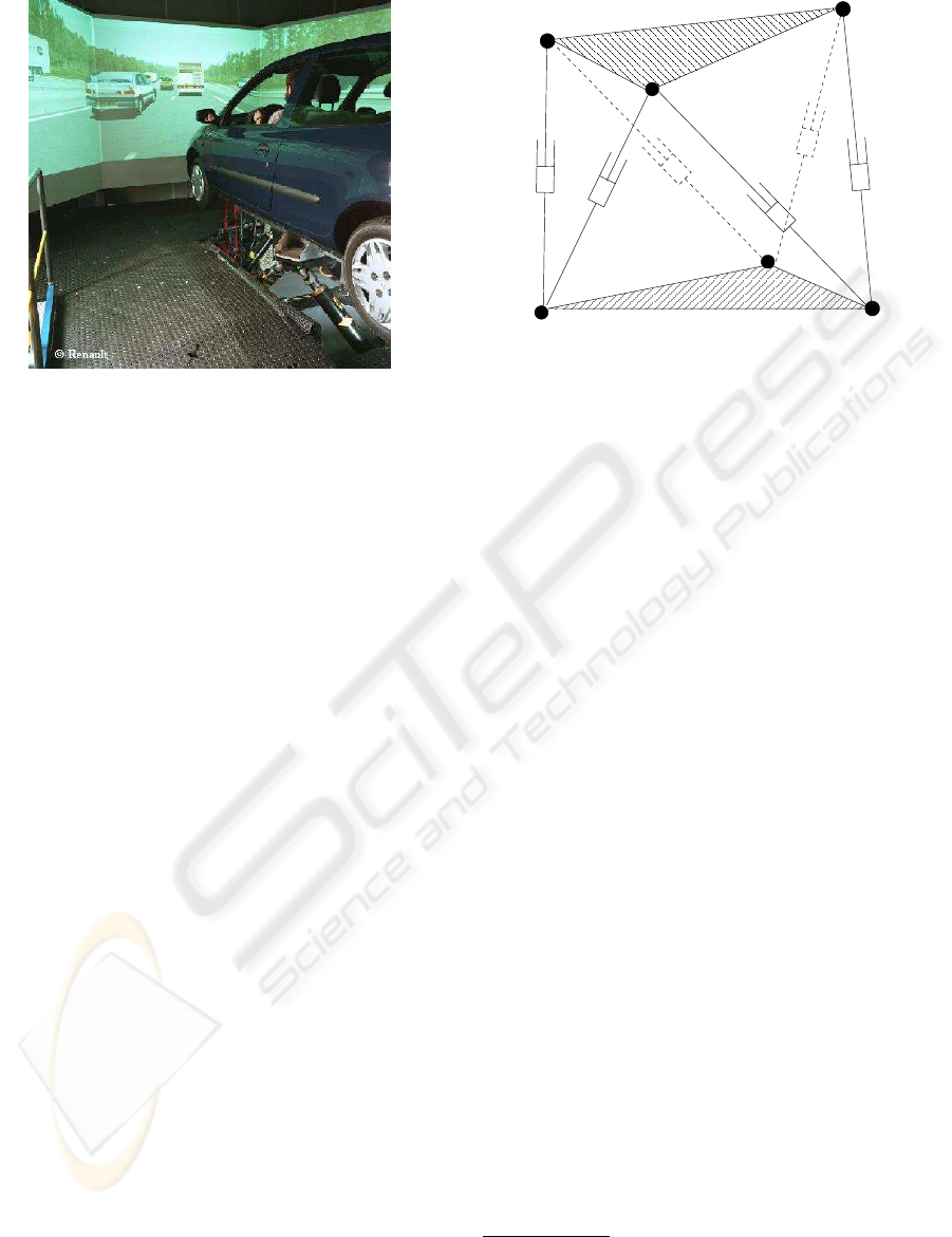
Figure 1: Renault dynamic simulator (Reymond et al, 2000)
The idea of this paper is to unify the washout block
with its tracking control neighbor in order to achieve
a better (global) optimization and to investigate the
nonlinear dynamics contribution.
The next sections will briefly introduce the reader
to the dynamics involved: the motion dynamics (the
platform, section II), the perception mechanism (the
vestibular system, section III). Then the formalization
section will figure out the details of the optimal mo-
tion cueing and will defend the authors approach.
Notation
• x or H: medium letters are scalars
• q: bold small letters are vectors
• M: bold capital letters are matrices
• ba: letters with a hat are perceived variables
2 PLATFORM KINEMATICS AND
DYNAMICS
The Gough-Stewart parallel robot is composed of
three parts: a moving body (the platform) linked
to a fixed body (the base) through six extensible
legs. Each leg is composed of a prismatic joint (i.e.
an electro-hydraulic jack) and two passive spherical
joints making the connection with the base and the
platform (Figure 2 depicts the platform without the
cockpit). For an excellent overview of parallel robots
the reader is referred to (Merlet, 2000).
Here the task space coordinates q are used to cal-
culate the dynamical model
q = [x, y, z, φ, θ, ψ]
T
(1)
Platform
Base
Figure 2: Parallel robot architecture
where (x, y, z) is the platform displacement vector
and (φ, θ, ψ) are the Euler angles defining its orien-
tation.
The Lagrange-Euler method was adopted to calcu-
late the 6-dimensional nonlinear system figuring the
generalized forces vector f
M(q)
¨
q + C(q,
˙
q)
˙
q + g(q) = f (2)
The symmetric positive semi-definite
2
matrix M(q)
is the mass tensor. C(q,
˙
q)
˙
q are the Coriolis and
centripetal forces (computed thanks to the Christoffel
symbols). g(q) are the gravity forces (including the
platform and the legs weights). Some usual simplifi-
cation hypotheses were put forward such as: friction
neglect, rigid bodies, and identical legs. The dynami-
cal model figuring the actuators forces u as the input
is obtained thanks to the relation (geometrical projec-
tion)
f = J
T
(q)u (3)
where J(q) is the inverse Jacobian matrix
3
.
Remark
The level of complexity of the dynamical model-
ing could be considered as a control parameter. In-
deed, some control problems could need high speed
processing, conflicting with a slow computational
model. The Lagrange-Euler method have an inter-
esting modular approach (based on the kinetic energy
separation). This property helps to build easily differ-
ent degree-of-complexity models.
2
The use of Euler angles induces purely mathematical
singularities at θ = ±π /2.
3
Singularity issues of the Jacobian matrix are not ad-
dressed in this paper (see (Merlet, 2000)).
AN OPTIMAL CONTROL SCHEME FOR A DRIVING SIMULATOR
41

Driving Simulator Optimal Control
Constrained Workspace, Nonlinear dynamics
Perception Error minimization
Real car
Trajectory
Real car
Trajectory
Real
Simulator
Trajectory
Optimal Motion
Cueing
Robot Tracking
Control
Desired
Simulator
Real car
Trajectory
Real car
Trajectory
Real
Simulator
TrajectoryTrajectory
Figure 3: Top diagram: the classical washout strategy. Bot-
tom diagram: the unifying optimal control strategy
3 THE VESTIBULAR SYSTEM
The vestibular system (VS), located in the inner ear, is
the inertial motion sensor. This biological apparatus
measures both linear and angular motions. The VS
is composed of two components: the otoliths and the
semicircular canals responsible respectively for lon-
gitudinal and for angular cue responses. More pre-
cisely, they are sensitive to linear acceleration and
to angular speed. An overview of these organs can
be found in (Berthoz and Droulez, 1982; Reymond,
2000). Otoliths have a noteworthy feature: they are
sensitive to the acceleration and to the gravity force
without the ability of distinction. The well-known
“tilt coordination”, for instance, uses this ambigu-
ity: “When a visual scene representing an accelerated
translation is presented to the driver while the simu-
lation cockpit is tilted at an undetectable rate, the rel-
ative variation of the gravity vector will be partly in-
terpreted as an actual linear acceleration” (Reymond
et al, 2000).
Vestibular models
For the longitudinal acceleration restitution (surge)
the adopted otoliths model is Telban’s (Telban and
Cardullo, 2001). It relates the perceived acceleration
ba (the hat means perceived) to the otoliths accelera-
tion:
ba
a
oto
=
K(τ
L
s + 1)
(τ
1
s + 1)(τ
2
s + 1)
(4)
The involved time constants are τ
L
= 10s, τ
1
= 5s
and τ
2
= 0.016s. K is a constant positive gain which
can be chosen arbitrarily. The otoliths acceleration
can be achieved either by translating the platform in
the surge direction x or by tilting it (following the
pitch angle θ)
a
oto
= ¨x − gθ (5)
The term ’−gθ’ is the ’tilt coordination’ contribution.
Note that the last equation is correct only for constant
angular speed and small angular motion.
The semi-circular model (Goldberg and Fernandez,
1971) relates the perceived angular speed bω to the
platform one ω =
˙
θ:
bω
ω
=
τ
a
τ
b
s
2
(τ
a
s + 1)(τ
b
s + 1)
(6)
The involved time constants are τ
a
= 5.7s and τ
b
=
80s.
4 OPTIMAL CONTROL
FORMALIZATION
This section first describes the optimal motion cueing
algorithm and then presents the authors extension and
contribution. The latter scheme is developed to study
offline platform responses, to check maneuvers feasi-
bility and to analyze the evolution and magnitudes of
the articular forces. In other words our approach does
not address real-time algorithms. Nonetheless it an-
swers the question: given the geometric constraints,
what is the best the platform can do?
4.1 Optimal motion cueing
Figure 4 summarizes the optimal washout scheme (re-
ferred to as washout in the following). Starting from
real car trajectories p
r
, one have (path 1) the motion
perception in a real world configuration. One have
as well (path 2) the motion perception caused by the
filtered trajectories p
s
(i.e. the trajectories that the
platform should track). The goal is to look for a lin-
ear washout filter W(s) that minimizes the perception
error i.e. the difference between these two paths.
The trajectories are represented by two parame-
ters: the linear acceleration and the angular speed.
Indeed they are the most significant factors for the
perception process (as described in section 3). Thus
p
r
= (a
r
, ω
r
) denotes the real car trajectory and
p
s
= (a
s
, ω
s
) is the trajectory that should be tracked
by the simulator.
The intuitive choice: “W(s) equals identity” gives
a perfect error cancellation. However, due to the plat-
form motion constraints this choice is not feasible.
The optimal motion cueing algorithm computes a lin-
ear washout filter W(s) by solving the following min-
imization problem: Given a filtered Gaussian noise as
a real car trajectory, minimize the statistical mean
min
p
s
E
Z
t
f
t
0
e
T
Qe + x
T
d
R
d
x
d
+ p
T
s
Rp
s
(7)
(The matrices involved in this cost are positive sym-
metric definite). This cost involves three terms:
• e
T
Qe: the perception error cost (perception valid-
ity)
ICINCO 2005 - ROBOTICS AND AUTOMATION
42

Perception
Filters
Washout
W(s)
Perception
Filters
+
−
Perception
Error
Real car
Trajectory
Real car
Trajectory
p
s
p
r
Path 2
Path 1
Trajectory
Simulator
Figure 4: Optimal motion cueing scheme
• x
T
d
R
d
x
d
: the platform displacement cost (con-
strained workspace). It is important to notice that
x
d
is ruled by a simple linear system. Indeed, it
is tacitly assumed that the platform tracks perfectly
the p
s
trajectories. Then x
d
is composed of the in-
tegrals of a
s
and ω
s
.
• p
T
s
Rp
s
: another way to account for the con-
strained workspace.
This algorithm has some drawbacks
• The washout block does not deliver the platform
trajectories but the ones that should be tracked.
Moreover, the tracking process will induce errors
and delays partly caused by the platform dynam-
ical delays and by the actuator coupling. And it
appears that it is more relevant and correct to min-
imize the perception error as a difference between
the tracked and the real perceived trajectories. This
is done in the unifying optimal control approach by
including a nonlinear dynamical model in the opti-
mization algorithm
• The actuator controls are constrained. However
these constraints are not directly included in the
washout algorithm. This may cause problems, for
instance: what if the desired trajectories are geo-
metrically feasible but the constraints on the con-
trols are not respected ?
• The washout algorithm does not use the ’tilt coor-
dination’. Indeed, for instance, if the real car per-
forms a linear acceleration, the trajectory delivered
by the washout will also be a linear simulator ac-
celeration (without any variation of the tilt angle)
• Motion cueing algorithms were primarily designed
for flight simulators. However “the dynamics of
land vehicle are very different the one of an air-
craft. Land vehicles are usually much faster if com-
pared to the one of a large aircraft. This is due to
a higher power to mass ratio and to the specific na-
ture of moving on the ground, where higher friction
is present” (Barbagli, 2001). This quick dynamics
(instantaneous breaks and accelerations) shows the
limitation of using a linear washout and motivates
exploring non-linear transformations.
4.2 Unifying optimal control
approach
In order to account for the last points, this paper uni-
fies the two blocks: control and washout filtering.
Thanks to the knowledge of the dynamical model (2),
(3) and the vestibular filters (4), (6), the authors pro-
pose to find the optimal actuator controls needed to
minimize
min
u
Z
t
f
t
0
e
T
Qe + x
T
d
R
d
x
d
+ u
T
Ru
(8)
Compared with the former cost (7)
• This is a deterministic approach. The goal is not
to find a washout filter, but to compute directly the
optimal actuator forces
• The perception error e is now the difference be-
tween the real simulator and the real car trajectories
• The displacement vector x
d
is ruled by the nonlin-
ear model (2): x
d
= (q,
˙
q)
• The cost p
T
s
Rp
s
is replaced by a cost on the actu-
ator forces u
T
Ru (so that one can act directly on
them)
Remarks
• Other choices of x
d
are possible. Indeed one can
select from (q,
˙
q) the relevant components with re-
spect to the experiment. For instance, in the case of
a pitch motion restitution, a possible choice of x
d
is (θ,
˙
θ), since the remaining degrees of freedom
should not be used.
• Besides the choice of the weights, this control is
parameterized by the dynamical model, the choice
of the vestibular filters, the choice of x
d
.
5 OPTIMAL CONTROL
CALCULATION AND
RESOLUTION
This section details the calculation and the resolution
of the optimal control problem. The whole system
(figuring the platform dynamics and the perception
mechanism) can be described by a first order system
with a linear dependence on u. Then, a simple the-
oretical expression for the optimal control u
∗
is ob-
tained. Eventually, the resolution scheme is formu-
lated as a boundary value problem.
AN OPTIMAL CONTROL SCHEME FOR A DRIVING SIMULATOR
43

5.1 Preliminaries
First of all, let us separate the control u into the effec-
tive control u
e
and the weight compensation control
u
g
:
u = u
e
+ u
g
, u
g
= J
−T
(q)g(q) (9)
Then, from (2) and (3) the new dynamical equations
involving u
e
are
J
−T
(q)M(q)
¨
q + J
−T
(q)C(q,
˙
q)
˙
q = u
e
(10)
This model is used to compute the optimal control.
Secondly, this second order system is converted to a
first order system with a new state variable
(x
1
, x
2
) = (q,
˙
q) (11)
˙
x
1
˙
x
2
=
x
2
a(x
1
, x
2
)
+
0
6×6
B(x
1
)
u
e
(12)
a and B are respectively a 6-dimensional vector and
matrix
a(x
1
, x
2
) = −M
−1
(x
1
)C(x
1
, x
2
)x
2
(13)
B(x
1
) = M
−1
(x
1
)J
T
(x
1
) (14)
Thanks to this linear dependence on u
e
, a simple the-
oretical expression for the optimal control is obtained.
Secondly, the robot is assumed to start from the initial
configuration q
0
4
. This initial point is a good esti-
mate of the 6-dimensional workspace center. Thirdly,
a 4-dimensional state-space representation is derived
from the vestibular filters (4) and (6) presented in sec-
tion 3:
˙
x
3
= A
ves
x
3
+ B
ves
(
˙
θ, ˙x)
T
(ba, bω)
T
= C
ves
x
3
+ D
ves
(
˙
θ, ˙x)
T
(15)
And finally the target is the final time t
f
. Let us define
the overall optimal control state variable
x = (x
T
1
, x
T
2
, x
T
3
)
T
(16)
The system then have a first order structure
˙
x = f (x) + G(x)u
e
(17)
Note that the drift dynamics f (x) (used in the last
equation) should not be confused with the generalized
forces f (in equation (2)).
5.2 Formalization
The overall cost to be minimized is as follows
J(x
0
, u
e
) =
Z
t
f
t
0
J
t
(x(t), u
e
(t), t)dt (18)
4
The neutral position q
0
can also be considered as a con-
trol parameter.
where the continuous criterion J
t
is the sum of
squared quadratic norms on the control magnitude,
the distance from the neutral configuration q
0
and the
perception error. Let’s define
x
d
= q − q
0
, e = (ˆa − ˆa
r
, ˆω − ˆω
r
)
T
(19)
(ˆa, ˆω) are the perceived acceleration and angular
speed provided by the platform whereas (ˆa
r
, ˆω
r
) are
the reference perceived trajectories i.e. the perception
of a real car trajectory. Then the cost is
J
t
= e
T
Qe + x
T
d
R
d
x
d
+ u
T
e
Ru
e
(20)
Writing the Hamiltonian
H = J
t
(x, u
e
) + λ
T
f(x) + λ
T
G(x)u
e
(21)
(λ is the 16-dimensional vector of the Lagrange multi-
pliers) shows its quadratic dependence on u
e
, thus al-
lowing a straightforward formula for the optimal con-
trol u
∗
e
u
∗
e
= −
1
2
R
−1
G
T
λ (22)
Eventually, the whole boundary value problem is
built. It consists of a 32-equation system:
˙
x = f (x) + G(x)u
∗
e
,
˙
λ = −
∂H
∂x
(x, λ, u
∗
e
, t) (23)
and the boundary conditions composed of the initial
and the transversality conditions
x(t
0
) = x
0
, λ(t
f
) = 0 (24)
6 SIMULATIONS
The Matlab
c
function ’bvp4c’ was used to solve this
boundary value problem. A passing maneuver was
simulated. A nonlinear platform dynamical model
with null-weighted legs was implemented.
Scenario
In the virtual world, the driver was provided prior mo-
tion and visual cues to give him the feeling of driving
at a constant speed. Now the robot is motionless at its
neutral position and the visual scene provides entirely
the motion illusion. Starting from this situation, the
driver accelerates to overtake a car and then deceler-
ates to restore his cruise speed. Two experiments were
carried out to simulate this manoeuvre: with and with-
out the use of the tilt coordination. Both tests used the
same weight matrices involved in the cost (8). These
weights were chosen so that, the platform can go near
to its displacement limits
5
. Consequently, they enable
a good exploitation of the simulator capabilities.
5
See the introduction section for the values.
ICINCO 2005 - ROBOTICS AND AUTOMATION
44
0 5 10 15 20
−2
−1.5
−1
−0.5
0
0.5
1
1.5
2
reference
washout
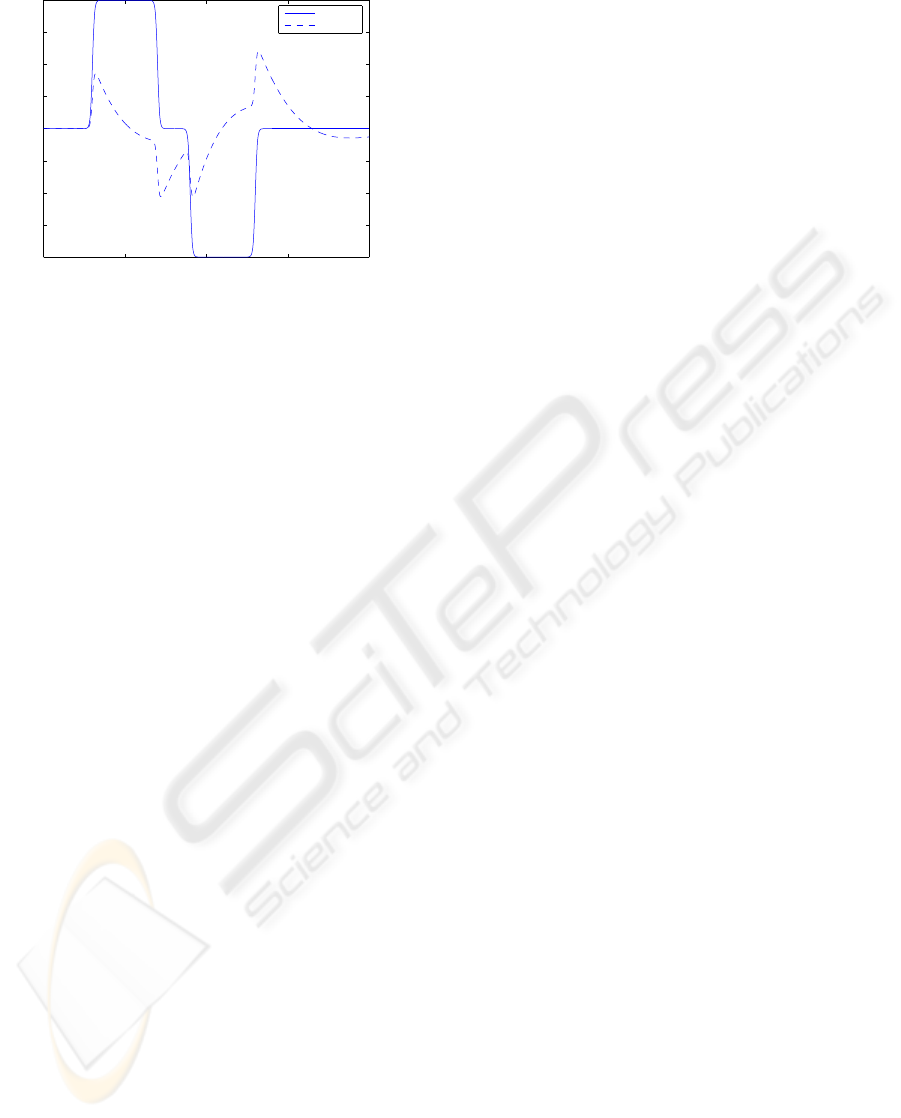
Figure 5: Real reference acceleration and washout acceler-
ation (ms
−2
)
Real values
This virtual scenario have a corresponding car trajec-
tory in the real world. Figure 5 depicts
• the real car acceleration trajectory a
r
(solid line).
The otoliths filter response to this trajectory is the
reference perception trajectory.
• the desired simulator trajectory a
s
delivered by the
washout (dashed line). This plot shows that the
washout is a high-pass filter that could induce sig-
nificant false cues (such as its responses at t = 7s
and t = 13s).
6.1 Without ’tilt coordination’
In this experiment, only the linear platform motion is
used to render the linear acceleration.
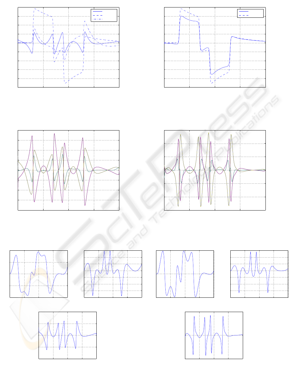
Comparing the motion perceptions
Figure 6 plots three perceived accelerations: the refer-
ence ba
r
, the optimal scheme ba (simulator, solid line)
and the washout ba
s
.
The authors scheme has three features:
• A backward platform motion (in ba) precedes the
desired forward one (see the first 3 seconds in
Fig.6). The platform goes back to perform bet-
ter forward acceleration. This could be explained
by the cost on the displacement x
T
d
R
d
x
d
(x
d
=
q − q
0
). Indeed it acts like a spring pulling the
simulator to its neutral position q
0
. The same com-
ment holds for the acceleration behavior at t = 9s.
• The optimal control scheme acts like a high-pass
filter. The sustained parts in the reference acceler-
ation ba
r
are completely canceled. This is natural
since the displacement is highly constrained.
• Thirdly, the optimal control amplitude is lesser than
the washout (dynamical limitation).
Other analysis
Figure 7 depicts the effective actuator forces u
∗
e
(with-
out the weight compensation forces). It presents fast
variations up to 350N. Figure 8 shows that the simu-
lator displacement, speed and acceleration are within
the constrained workspace.
Conclusion The constrained workspace altered
considerably the rendering of the acceleration percep-
tion.
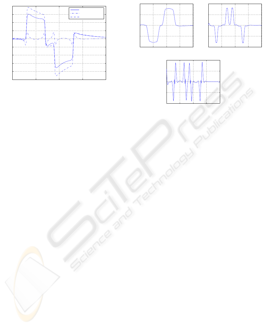
6.2 With ’tilt coordination’
In this simulation, both linear motion and tilt coordi-
nation were used to render the linear acceleration.
Comparing the motion perceptions
Figure 9 shows an excellent rendering of the accel-
eration perception. The ’tilt coordination’ is indeed
essential in this experiment. The tilt contributes con-
siderably to the perception (Fig.12) despite a very re-
duced angular motion (Fig.13). It enables the restitu-
tion of the low-frequency part that could not be per-
formed by the linear motion.
Other analysis
As the ’tilt coordination’ shares the restitution task
with the linear motion, the latter have lesser ampli-
tudes (see Fig.11) than the former test (without tilt).
The actuator controls are lesser as well (see Fig.10).
Conclusion The ’tilt coordination’ is a powerful
trick to circumvent the workspace constraints. Very
good results are achieved.
7 CONCLUSION
The purpose of the this paper is to develop an opti-
mal control approach that extends and over-perform
the optimal motion cueing algorithm. A nonlinear dy-
namical model was built. Vestibular filters and the ’tilt
coordination’ trick were included in the algorithm.
Simulations showed the influence of the nonlinear dy-
namics and the importance of ’tilt coordination’. Fu-
ture works will deal with the vestibular-visual interac-
tion. Robustness shall also be studied by integrating
modelling errors and computation delays.
AN OPTIMAL CONTROL SCHEME FOR A DRIVING SIMULATOR
45
0 5 10 15 20
−5
−4
−3
−2
−1
0
1
2
3
4
simulator
reference
washout
Figure 6: No tilt: perceived accelerations
0 5 10 15 20
−400
−300
−200
−100
0
100
200
300
400
Figure 7: No tilt: u
∗
e
actuator forces N
0 5 10 15 20
−0.2
−0.1
0
0.1
0.2
(a)
0 5 10 15 20
−0.4
−0.3
−0.2
−0.1
0
0.1
0.2
0.3
(b)
0 5 10 15 20
−1
−0.5
0
0.5
1
(c)
Figure 8: No tilt: (a) platform displacement m, (b) platform
speed ms
−1
, (c) platform acceleration ms
−2
0 5 10 15 20
−5
−4
−3
−2
−1
0
1
2
3
4
simulator
reference
Figure 9: With tilt: perceived accelerations
0 5 10 15 20
−300
−200
−100
0
100
200
300
Figure 10: With tilt: u
∗
e
actuator forces N
0 5 10 15 20
−0.05
0
0.05
(a)
0 5 10 15 20
−0.2
−0.15
−0.1
−0.05
0
0.05
0.1
0.15
(b)
0 5 10 15 20
−0.5
0
0.5
(c)
Figure 11: With tilt: (a) platform displacement m, (b) plat-
form speed ms
−1
, (c) platform acceleration ms
−2
ICINCO 2005 - ROBOTICS AND AUTOMATION
46
0 5 10 15 20
−5
−4
−3
−2
−1
0
1
2
3
4
tilt coordination
linear acceleration
reference
Figure 12: With tilt: linear acceleration and tilt coordination
contributions to the perception restitution
ACKNOWLEDGMENT
This work has been supported by the French ministry
of transportation in the framework of the PREDIT
programme 2002-2006: HybriSim project.
REFERENCES
Barbagli, F. et al (2001). Washout filter design for a motor-
cycle simulator. In IEEE Computer Society, Proceed-
ings of the Virtual Reality 2001 Conference, pages
225–232, Yokohama, Tokyo.
Berthoz, A. and Droulez, J. (1982). Linear self-motion
perception. Tutorials on Motion Perception, A.H.
Wertheim, W.A. Wagenaar and H.W. Leibowitz (eds.),
Plenum, New York.
Cardullo, F.M. et al (1999). Motion cueing algorithms: A
human centered approach. 5th International Sympo-
sium on Aeronautical Sciences, Zhukovsky, Russia.
Goldberg, J. and Fernandez, C. (1971). Physiology of pe-
ripheral neurons innervating semicircular canals of the
squirrel monkey. ii. response to sinusoidal stimulation
and dynamics of peripheral vestibular system. Journal
of Neurophysiology, 34:661–675.
Guo, L. et al (2003). The results of a simulator study to
determine the effects on pilot performance of two dif-
ferent motion cueing algorithms and various delays,
compensated and uncompensated. American Institute
of Aeronautics and Astronautics: Modeling and Sim-
ulation Technologies Conference and Exhibit, Austin,
Texas.
Merlet, J.-P. (2000). Parallel Robots, volume 74 of Solid
mechanics and its applications. G.M.L. Gladwell
(ed), Kluwer Academic Publishers.
Reymond, G. et al (2000). Validation of Renault dy-
namic simulator for adaptive cruise control experi-
0 5 10 15 20
−0.2
−0.1
0
0.1
0.2
(a)
0 5 10 15 20
−0.2
−0.1
0
0.1
0.2
(b)
0 5 10 15 20
−0.4
−0.2
0
0.2
0.4
(c)
Figure 13: With tilt: (a) tilt angle rd, (b) tilt speed rds
−1
,
(c) tilt acceleration r ds
−2
ments. Proceedings of the Driving Simulation Con-
ference, pages 181–191, Paris.
Reymond, G. (2000). Contribution des stimulis visuels,
vestibulaires et proprioceptifs dans la perception du
mouvement du conducteur. PhD thesis, Neurosciences
department, Universit
´
e Paris VI - Renault.
Telban, R.J. et al (1999). Developments in human centered
cueing algorithms for control of flight simulator mo-
tion systems. American Institute of Aeronautics and
Astronautics: Modeling and Simulation Technologies
Conference and Exhibit, Portland. OR.
Telban, R.J. and Cardullo, F.M. (2001). An integrated
model of human motion perception with visual-
vestibular interaction. American Institute of Aeronau-
tics and Astronautics: Modeling and Simulation Tech-
nologies Conference and Exhibit, Montreal, Canada.
Telban, R.J. and Cardullo, F.M. (2002). A nonlinear,
human-centered approach to motion cueing with a
neurocomputing solver. American Institute of Aero-
nautics and Astronautics: Modeling and Simulation
Technologies Conference and Exhibit, Monterey, Cal-
ifornia.
AN OPTIMAL CONTROL SCHEME FOR A DRIVING SIMULATOR
47
