
A New Training Algorithm for Neuro-Fuzzy Networks
Stefan Jakubek
1
and Nikolaus Keuth
2
1
Vienna University of Technology,
Institute for Mechanics and Mechatronics,
Gußhausstr. 27-29/E325, A-1040 Vienna, Austria
2
AVL List GmbH, Hans-List Platz 1, A-8020 Graz , Austria,
Abstract. In this paper a new iterative construction algorithm for local model
networks is presented. The algorithm is focussed on building models with sparsely
distributed data as they occur in engine optimization processes. The validity func-
tion of each local model is fitted to the available data using statistical criteria
along with regularisation and thus allowing an arbitrary orientation and extent
in the input space. Local models are consecutively placed into those regions of
the input space where the model error is still large thus guaranteeing maximal
improvement through each new local model. The orientation and extent of each
validity function is also adapted to the available training data such that the de-
termination of the local regression parameters is a well posed problem. The reg-
ularisation of the model can be controlled in a distinct manner using only two
user-defined parameters. Examples from an industrial problems illustrate the ef-
ficiency of the proposed algorithm.
1 Introduction
Modeling and identification of nonlinear systems is challenging because nonlinear proc-
esses are unique in the sense that they may have an infinite structural variety compared
to linear systems. A major requirement for a nonlinear system modeling algorithm is
therefore universalness in the sense that a wide class of structurally different systems
can be described.
The architecture of local model networks is capable of fulfilling these requirements
and can therefore be applied to tasks where a high degree of flexibility is required. The
basic principles of this modeling approach have been more or less independently de-
veloped in different disciplines like neural networks, fuzzy logic, statistics and artificial
intelligence with different names such as local model networks, Takagi-Sugeno fuzzy
models or neuro-fuzzy models [1–5].
Local model networks possess a good interpretability. They interpolate local mod-
els, each valid in different operating regions, determined by so-called validity functions.
Many developments are focused on the bottleneck of the local model network which is
the determination of these subdomains or validity functions, respectively.
One important approach is Fuzzy clustering as presented in [6, 1,7, 8]. An important
issue in this field is the interpretability of the validity functions, for example as operating
regimes. Recent developments can be found for example in [9, 10].
Jakubek S. and Keuth N. (2005).
A New Training Algorithm for Neuro-Fuzzy Networks.
In Proceedings of the 1st International Workshop on Artificial Neural Networks and Intelligent Information Processing, pages 23-34
DOI: 10.5220/0001180200230034
Copyright
c
SciTePress

Another development is the local linear model tree, LOLIMOT [11]. It is based
on the idea to approximate a nonlinear map with piece-wise linear local models. The
algorithm is designed such that it systematically bisects partitions of the input space.
Local models that do not fit sufficiently well are thus replaced by two or more smaller
models in the expectation that they will fit the nonlinear target function better in their
region of validity.
In the practical application that motivated this work the amount of data available
for identification is limited and the distribution of the data in their input space is sparse
[12]. This imposes a limit on the network construction algorithm and it can lead to the
situation that many local models are built where much fewer would be sufficient. Also,
the sparseness of the input data gives rise to a more or less automated regularization
that can be handled even by inexperienced users. The local model network construction
algorithm presented in this paper can be seen as a mixture of classical fuzzy clustering
techniques and the LOLIMOT construction algorithm. The present clustering algorithm
takes into account the spatial distribution of the data in the input space and the prospec-
tive shape of the target function. The extent of the local model in the input space and its
orientation are determined such that maximal statistical consistency/compliance with
the sample data is achieved along with a spatial distribution of the data that yields a
well conditioned problem.
The efficiency of the training algorithm is thus significantly increased resulting in
less computational effort and fewer local models.
2 Algorithm Description
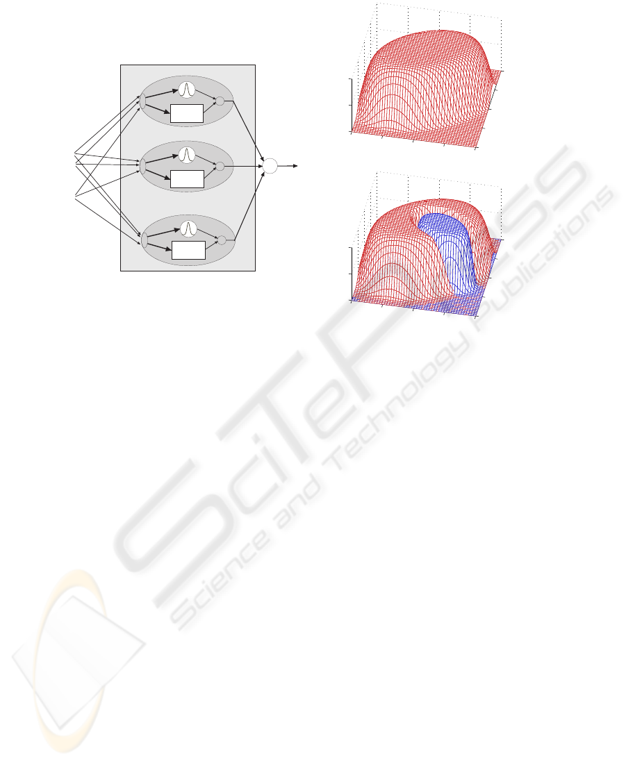
Fig. 1 illustrates the architecture of a local model network. Each local model (denoted
as LM
i
) takes the input vector u = [ u
1
u
2
. . . u
q
]
T
to compute its associated
validity function Φ
i
and its local estimation ˆy
i
of the nonlinear target function f(u).
The aggregate network output is the sum of all local model outputs ˆy
i
:
ˆy(u) =
m
X
i=1
Φ
i
(u)ˆy
i
(u, θ
i
) (1)
Here, θ
i
is a vector containing the parameters of the local model and the local model
output is generated from u and θ
i
.
The structure of the validity function Φ
i
was chosen as
Φ
i
(u) = exp
−[(u − z
i
)
T
A
i
(u − z
i
)]
κ
i
·
m
Y
k=i+1
(1 − Φ
k
(u)) (2)
The vector z
i
contains the location of the current local model center, A
i
is a sym-
metric and positive definite matrix that determines the orientation and extent of the va-
lidity function in the input space and the exponent κ
i
is a shape factor that determines
the flatness of the validity function and thus also the degree of overlap between different
local models. In the given examples this factor was set to 4, a further discussion on the
choice of κ follows.
24
X
X
X
+
.
.
.
.
.
.
u
1
u
2
u
j
u
u
u
Φ
1
Φ
2
Φ
m
ˆy
1
ˆy
2
ˆy
m
ˆy
LM
1
LM
2
LM
m
Fig.1. Concept of local model networks
−0.5
0
0.5
1
1.5
−0.5
0
0.5
1
1.5
0
0.5
1
u
1
u
2
Φ
i
(u
1
, u
2
)
−0.5
0
0.5
1
1.5
−0.5
0
0.5
1
1.5
0
0.5
1
u
1
u
2
Φ
i
(u
1
, u
2
)
Fig.2. Shape and hierarchy of validity functions
The structure of eq. (2) shows that every validity function is initally an exponential
function with ellipsoidal contour lines. The product in (2) clips all subsequent validity
functions from this original function, see Fig. 2. This choice has the following advan-
tage: All subsequent local models are set into domains of the input space, where the
preexisting model is insufficient. Eq. (2) ensures the dominance of the new local mod-
els in such domains. In Fig. 2 the situation is illustrated for a two-dimensional input
space where a small domain is clipped from an originally ellipsoidal validity function.
The structure of (2) by iteself does not guarantee that validity functions yield a
partition of unity. For that purpose the validity functions are normalized which is not
explicitly oulined here for the sake of brevity.
The overall quality of the network output is assessed either by the R
2
statistics or
by the R
2
pred
statistics as outlined in [13]. The R
2
pred
statistics inherently describes the
generalization quality of the model.
2.1 Training procedure
The local model network construction algorithm consists of an outer loop that deter-
mines the location, extent and orientation of each local model and a nested inner loop
that optimises the parameters of the local model:
1. Start with an initial model: The initial model can either be a global model that
covers all the available data or an ”ordinary” local model as described below.
25

2. Set the next local model: Find the data point with the worst output error or predic-
tion error. Choose the location of this data point as a candidate for the next local
model. Design the orientation and extent of the new model such that it meets sta-
tistical compliance criteria with the sample data in the region of its validity. This
procedure will be described in detail in the next section.
3. Compute the local model parameters and the associated statistical parameters that
are necessary for the computation of prediction intervals
4. Test for Convergence: The performance criteria R
2
and R
2
pred
for the network out-
put are computed. Once they have reached or exceeded their termination values the
algorithm stops. Also, if no further improvement can be achieved the tree construc-
tion is stopped. Otherwise the algorithm proceeds with step 2. Especially in the
case when the training data are subject to strong noise disturbance it is important
that the training algorithm is controlled by a useful regularisation factor. Otherwise,
the construction algorithm would create smaller and even smaller local models to
improve the overall fit. In our case this is prevented by means of confidence levels
as will be described in detail in the next section.
After the local model network construction algorithm has finished to place local
models each model undergoes a final examination for its contribution to the overall
network output. If it turns out that a certain model does not contribute significantly
anymore because it has been replaced by other models to a great extent it is removed.
3 Local Model Design
3.1 Local Model Structure
Every local model roughly consists of two parts: Its validity function Φ
i
(u) and its
model parameters θ
i
. The output ˆy
i
of a local model at a point u in the input space is
chosen as
ˆy
i
(u) = x
T
(u) · θ
i
. (3)
Here, x
T
(·) represents a row vector of regressor functions which can be chosen ar-
bitrarily. The advantage of the structure of (3) lies in the fact that ˆy
i
depends linearly
on the parameters θ
i
. Therefore, least-squares techniques can be applied for their com-
putation. It remains to determine suitable regressor functions for x
T
(·) which will be
outlined in section 3.3.
3.2 Determination of the validity function
In the presence of noise it is desirable that every local model should have optimal sta-
tistical significance. The algorithm presented in the sequel takes into account both the
spatial distribution of the data and the expected shape of the target function and how
well it can be modeled by the given regressors. In practical situations both the effect of
noise and the prospective shape of the target function are unknown and the presented
clustering approach turned out to be a reliable compromise.
26

1. The selection of a center ”candidate” z
i
of a new local model is based on the
estimation error e
j
= y
j
− ˆy(u
j
). Here ˆy(u
j
) is the model output from the network
at it’s current state when i − 1 models have already been built:
ˆy(u
j
) =
i−1
X
k=1
Φ
k
(u
j
)ˆy
k
(u
j
, θ
k
) (4)
Given n data records u
j
for model training the new center candidate is chosen as
the data record where the output error is maximal:
z
i,cand
= u
j
m
with j
m
= arg max ||e
j
|| (5)
This selection ensures that a new local model is set in the area where it is needed
most.
2. Next, an initial set of neighbouring training data is chosen to compute an ”initial”
regression model. The minimum amount of data necessary for this initial model
is determined by the requirement that the regression matrix must have maximum
rank which depends both on the regressor functions and on the spatial distribution
of the data. Next, the model statistics of the regression model are computed (see
sec. 3.4) and a check is performed whether the initial data set lies within a pre-
scribed prediction interval corresponding to a confidence level α. If this is not the
case the iteration terminates and the algorithm proceeds with the computation of
the parameters of the validity function. Typically, the confidence level α is chosen
between 90% and 99.9%.
3. Otherwise, further training data points in the vicinity of z
i,cand
are added succes-
sively and the initial regression model together with the model statistics are adapted
to these data using recursive least squares techniques. This step is repeated as long
as α % of the selected training data lie within the prediction interval. Thus it is
ensured that the local model size and shape corresponds to the shape of the target
function and the noisyness of the data.
4. Once training data have been selected in this way their distribution in the input
space is used to determine the actual center along with the shape and extent of the
validity function.
Figures 3 and 4 give an example for a nonlinear map f(u) : IR → IR and α = 97%.
The training data are represented by dots. Figure 3 depicts an ”initial” regression model:
The center candidate was chosen as z
i,cand
= 0 for this illustrative example, all data
points in the interval u ∈ [0; 0.17] were selected for the regression. The dashed curves
represent the boundaries of the 97% prediction interval. Figure 4 depicts the ”final” sit-
uation: Additional training data points had been added until finally about 97% of the
selected data lie within the boundaries of the 97% confidence interval. The resulting
validity function which was added to the figure for clarity extends from 0.1 to 0.8 hav-
ing its maximum at 0.4. Figure 5 illustrates the final situation for α = 99.99%. The
increased confidence level α results in larger confidence intervals and consequently the
validity function now has a greater extent. It can also be seen that in this example the
shape of the nonlinearity has a much greater influence on the model size than in Figure
27
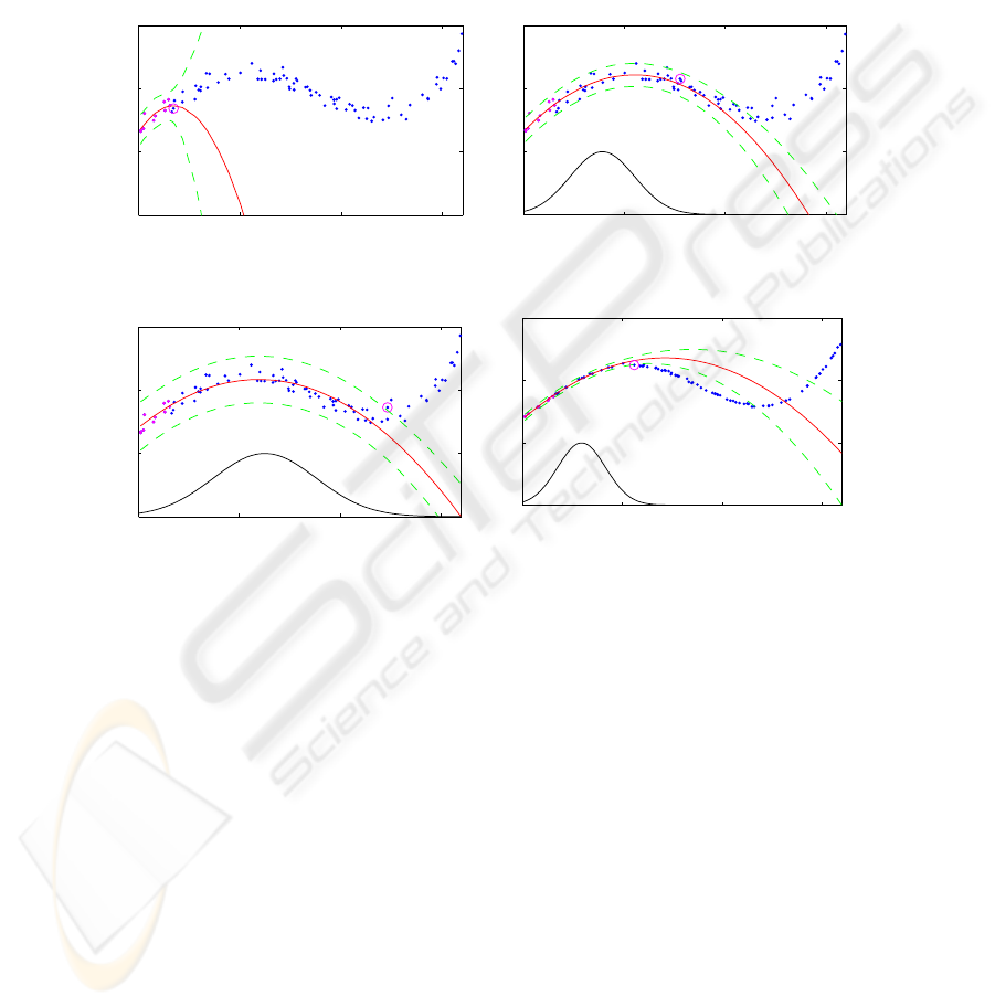
4. Figure 6 contains the same map f(x), however, the influence of noise was drasti-
cally reduced. Altough the confidence level is still at 99.99% the extent of the validity
function is now significantly smaller. From these examples it becomes obvious that the
confidence level α serves as an excellent regularisation parameter that automatically
adapts the local models to the noise corruption of the training data and to the regressor
functions.
0 0.5 1 1.5
0
1
2
3
u
Φ(u), y, ˆy
Fig.3. Initial model with α = 97%
0 0.5 1 1.5
0
1
2
3
u
Φ(u), y, ˆy
Fig.4. Final local model with α = 97%
0 0.5 1 1.5
0
1
2
3
u
Φ(u), y, ˆy
Fig.5. Final local model with α = 99.99%
0 0.5 1 1.5
0
1
2
3
u
Φ(u), y, ˆy
Fig.6. Final local model with α = 99.99% and
less noise
It remains to determine the nonlinear parameters of the validity function from the
training data selected in the manner described above. Let U
sel
be a matrix containing
all these data records including the center candidate z
i
, i.e. every row vector of U
sel
contains the coordinate vector u
i
of a selected data point.
Then, the actual center is obtained by taking the center of gravity of the data in
U
sel
:
z
i
= mean(U
sel
) (6)
where mean(·) takes the mean value over every column of its argument. The actual
center is thus not the initial center candidate but the center of gravity of all chosen data
points. This has the advantage that the algorithm is less sensitive to outliers in the data
set.
28

The matrix A
i
is computed by
A
i
= γ · [cov(U
sel
)]
−1
(7)
where cov(·) denotes the empirical covariance matrix. This approach is taken from [14]
where it was applied for the design of ellipsoidal basis function networks. The principal
orientation of the new validity function is thus determined by [cov(U
sel
)]
−1
and its
extent in the input space is controlled by γ. The latter is chosen such that Φ
i
is still 0.9
at the data point in U
sel
which is located most remote from the new center z
i
. Thus, it
is ensured that there are actually enough data points available for parameter estimation.
Besides α, both γ and the shape parameter κ constitute a second means of regularisation
for the algorithm. The larger κ is chosen the smaller the overlap between single local
models will be. Thus κ directly controls the locality of the models. This does play an
important role in the determination of covariances as will be outlined later. The factor
γ is directly related to the choice of κ and just has to ensure the LS-problem is well
posed as stated earlier. Consequently, the confidence level α and κ are used to tune the
training algorithm.
3.3 Computation of the local model parameters
As already mentioned earlier the output of each local model is computed through the
regression model (3). It remains to determine suitable regression functions x
T
(u). In
general, there is no ”optimal” solution that suits all possible nonlinear problems. The
LOLIMOT-Algorithm [11] features linear models and in the present application the
regressor functions were chosen as quadratic polynomials.
Let X denote a matrix constructed from the regression vectors of all n training data
records:
X =
x
T
(u
1
)
x
T
(u
2
)
.
.
.
x
T
(u
n
)
and Q
i
=
Φ
i
(u
1
) 0 · · · 0
0 Φ
i
(u
2
) · · · 0
.
.
.
.
.
.
.
.
.
.
.
.
0 0 · · · Φ
i
(u
n
)
(8)
where Q
i
denotes a diagonal matrix composed from the Φ
i
, evaluated at the training
data points. If y is a vector containing the values of the target function at the data points
then the i-th local parameter vector is given by
θ
i
=
X
T
Q
i
X
−1
X
T
Q
i
y. (9)
3.4 Local Model Statistics
Using the abbreviation
Θ
Q
=
X
T
Q
j
X
−1
(10)
the parameter variance cov(θ) can be expressed by
29

cov(θ) = σ
2
n
Θ
Q
X
T
Q
2
i
XΘ
Q
. (11)
with the assumption that the measurement noise at different training data points is un-
correlated E{ee
T
} = σ
2
n
I. It has to be mentioned that the noise covariance σ
2
n
is
not known in most cases and therefore has to be replaced by the empirical covariance
computed from the available data.
The variance of the local model output ˆy
i
(u
i
) is then calculated by
cov(ˆy
i
(u)) = E
(y
i
− ˆy
i
)
2
== σ
2
n
[1 + x(u
i
)Θ
Q
X
T
Q
2
i
XΘ
Q
x
T
(u
i
)]. (12)
The prediction interval at a point u in the input space with a significance level of α
is given by
|ˆy(u) − y(u)|
α
= σ
n
q
1 + x(u)Θ
Q
X
T
Q
2
j
XΘ
Q
x(u)
T
× t
1−
α
2
(13)
As indicated, the t-statistics have to be computed for a significance level of α-%
with the degrees of freedom depending on both the number of training data involved
and the number of regressors.
4 Global Model Design
Apart from the local model design the interaction of all local models has to be consid-
ered in a global design. This involves the aggregation of the local model outputs as well
as global model statistics, global prediction intervals and efficient ways to compute the
R
2
and R
2
pred
statistics.
4.1 Global Model Output
As defined in (1) the global model output is a weighted sum of all local outputs. The
weights depend on the location u in the input space and are determined from the validity
functions Φ:
ˆy(u) =
m
X
i=1
Φ
i
(u)ˆy
i
(u, θ
i
)
As already mentioned earlier the design parameters of the validity function, κ in
particular implicitly determine the degree of overlap between the local models and thus
serve as a regularisation parameter. It is straightforward that strong overlap in general
leads to smoother function approximation.
30

4.2 Global Prediction Intervals
Computation of confidence intervals at the global level involves two steps:
1. Computation of the covariance
2. Determination of the effective degrees of freedom at the global level for the t
α
statistics.
Step 1 is straightforward since the global model output is a linear combination of
the local model as given by (1). Strictly speaking, the outputs of different local models
ˆy
i
(u) are not independent since the underlying models all originate from the same data.
However, the shape parameter κ in (2) entails that there is only little overlap between
single local models. The statistical interdependencies between local models is therefore
neglegible, which was also verified in numerous tests.
cov(ˆy(u)) =
m
X
i=1
Φ
2
i
(u)cov(ˆy
i
(u)) (14)
In the above formula cov(ˆy
i
(u)) is taken from (12). It is noteworty that (14) does
not contain σ
2
n
directly. The covariance cov(ˆy
i
(u)) of every local model depends on the
model structure and on the local measurement noise. This means that (14) could also be
applied if the measurment noise varies from local model to local model, provided that
cov(ˆy
i
(u)) is computed correctly.
Step 2 is taken from [5] where the effective number of parameters n
eff
is deter-
mined from the trace of the so-called ”smoothing matrix”.
The remaining degrees of freedom then result to D OF = n − n
eff
and this is the
basis for the computation of the t-statistics. It is noteworthy that n
eff
is not necessarily
an integer number. During the tree construction process it sometimes happens that the
validity function of a certain local model is successively clipped away by subsequent
models so that it finally doesn’t contribute anymore to the model quality. In the present
application these models are finally removed if their n
eff,i
has dropped below 1.
5 Results
In the given example measurement data from an IC-Engine are considered. For the de-
velopment and testing of the presented algorithm measurement databases from different
engine manufacturers were used. The dimension of the input space in these databases
varies from three to eight.
The three-dimensional database will be illustrated in detail since in this case some
demonstrative graphical illustrations can be given.
In particular, the air efficiency A
e
of a valvetronic engine shall be represented as a
function of engine speed n, valve lift L
v
and intake closure time T
c
:
A
e
= f (n, L
v
, T
c
)
31
The resulting network models the map f : IR
3
→ IR with an accuracy of R
2
=
0.9941 and R
2
pred
= 0.9931 using 7 local models. In comparison, the LOLIMOT-
algorithm using the same quadratic local model structure needs 30 local models to reach
the same accuracy.
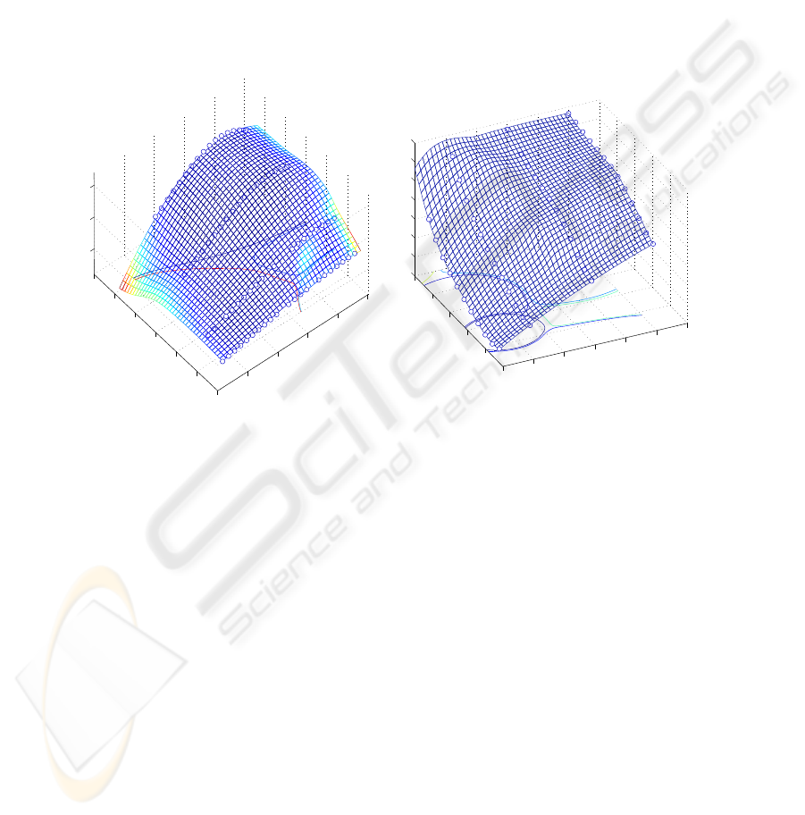
Figures 7, 8 and 9 depict the network output each with one input kept constant.
Apart from the network output the corresponding training data points are depicted and
the validity functions are represented by contour lines. Note that not all seven validity
functions are visible in the respective intersection planes. It can be seen that they are
fitted to the shape of the target function in an efficient way.
400
450
500
550
600
650
1
2
3
4
5
6
7
0
0.5
1
T
c
L
v
Fig.7. Valvetronic engine example: Model out-
put for n = 2600 =const.
1000
2000
3000
4000
5000
60001
2
3
4
5
6
7
0
0.1
0.2
0.3
0.4
0.5
0.6
0.7
n
L
v
Fig.8. Valvetronic engine example: Model
output for T
c
= 498 =const.
The measurement data considered in this example were also used to compare the
performance of the presented network architecture and training algorithm to that of a
perceptron network. The number of hidden neurons was chosen such that the effective
number of weights corresponds to the number of parameters in the competing local
model network. The weights of the perceptron network were optimized using standard
training algorithms in combination with different regularization techniques in order to
balance bias and variance errors. In a Monte-Carlo simulation it turned out that despite
this efforts the perceptron has particular difficulties interpolating the large gaps between
the individual valve lift values (cf. Fig. 7 and Fig. 10).
Altogether, 300 Perceptrons were trained in the manner described above, resulting
in the following statistical assessment: 13% of all Perceptrons had a performance supe-
rior to that of the local model network. They exceeded the R
2
pred
value of 0.9931 and the
interpolation behaviour was better. 13% of all Perceptrons produced a comparable per-
formance in terms of the same criteria. The remaining 74% of all 300 perceptrons were
32

450
500
550
600
650
1000
2000
3000
4000
5000
6000
−0.5
0
0.5
1
1.5
T
c
n
Fig.9. Valvetronic engine example: Model
output for L
v
= 6 =const.
400
500
600
700
0
2
4
6
−1
0
1
2
T
c
L
v
Fig.10. Valvetronic engine example: Percep-
tron output for n = 2600 =const.
outperformed by the local model network, cf. Fig. 10. In many cases the confidence
interval was unacceptably large for practical applications.
6 Conclusion and Outlook
In this paper a new iterative tree construction algorithm for local model trees was pre-
sented. The validity functions of the generated model are closely fitted to the available
data by allowing an arbitrary orientation and extent of the validity function of each local
model in the input space.
The regularisation of the model can be controlled by a shape factor κ which deter-
mines the overlap between local models and by a confidence level α that controls the
relative size of each local model.
The application to data from internal combustion engines shows that the proposed
algorithm produces excellent results with a relatively low number of local models.
References
1. Babuska, R., Verbruggen, H.: An overview of fuzzy modeling for control. control Engineer-
ing Practice 4 (1996) 1593 – 1606
2. Johansen, T.A., Foss, B.A.: Operating regime based process modeling and identification.
Computers and Chemical Engineering 21 (1997) 159 – 176
3. Babuska, R.: Recent Advances in Intelligent Paradigms and Applications. Springer-Verlag,
Heidelberg (2002)
4. Ren, X., Rad, A., Chan, P., Wai, L.: Identification and control of continuous-time nonlin-
ear systems via dynamic neural networks. Industrial Electronics, IEEE Transactions on 50
(2003) 478–486
5. Nelles, O.: Nonlinear System Identification. 1st edn. Springer Verlag (2002)
33

6. Bezdek, J., Tsao, E.K., Pal, N.: Fuzzy kohonen clustering networks. In: IEEE International
Conference on Fuzzy Systems, IEEE (1992) 1035 – 1043
7. Yen, J., L., W.: Application of statistical information criteria for optimal fuzzy model con-
struction. IEEE Transactions on Fuzzy Systems 6 (1998) 362 – 372
8. Gath, I., Geva, A.: Unsupervised optimal fuzzy clustering. IEEE Transactions on Pattern
Analysis and Machine Intelligence 11 (1989) 773–781
9. Abonyi, J., Babuska, R., Szeifert, F.: Modified gath-geva fuzzy clustering for identification
of takagi-sugeno fuzzy models. In: IEEE Tarnsactions on systems, man. and Cybernetics.
Volume 32., IEEE (2002) 612–621
10. Trabelsi, A., Lafont, F., Kamoun, M., G., E.: Identification of nonlinear multivariable systems
by adaptive fuzzy takagi-sugeno model. International Journal of Computational Cognition
(http://www.YangSky.com/yangijcc.htm) 2 (2004) 137–153
11. Nelles, O., Isermann, R.: Basis function networks for interpolation of local linear models.
In: IEEE Conference on Decision and Control (CDC). (1996) 470–475
12. Bittermann, A., Kranawetter, E., J., K., B., L., T., E., Altenstrasser, H., Koegeler, H.,
Gschweitl, K.: Emissionsauslegung des dieselmotorischen fahrzeugantriebs mittels doe und
simulationsrechnung. Motorentechnische Zeitschrift (2004)
13. Hong, X., Sharkey, P., Warwick, K.: A robust nonlinear identification algorithm using press
statistics and forward regression. In: IEEE Transactions on Neural Networks. Volume 14.,
IEEE (2003) 454 – 458
14. Jakubek, S., Strasser, T.: Artificial neural networks for fault detection in large-scale data
acquisition systems. Engineering Applications of Artificial Intelligence 17 (2004) 233–248
34
