
GENETIC AND ELLIPSOID ALGORITHMS FOR NONLINEAR
PREDICTIVE CONTROL
Kaouther Laabidi
High Institute of Applied Sciences and Technology, Mateur, Tunisia.
Faouzi Bouani, Mekki Ksouri
National Institute of Applied Sciences and Technology, Tunis, Tunisia
Keywords: Predictive control, constraints, nonlinear systems, genetic algorithms, ellipsoid algorithm.
Abstract: This paper deals with the constrained predictive control of nonlinear systems. Artificial Neural Networks
(ANN) are used as a process model. The control law is derived by minimizing a non convex criterion. The
optimization problem is solved using Ellipsoid and genetic algorithms. The structure and operators of the
combining two algorithms have been specifically developed for control design problem. Simulation results
are presented to illustrate the performances of the proposed predictive controller.
1 INTRODUCTION
Several dynamical systems are provided of non
linearity with significant uncertainty which have
limited the use of linear model based predictive
controllers. Consequently, nonlinear predictive
controllers are developed based on a nonlinear
process model. The use of a nonlinear model leads
to a non convex optimization problem which is
generally hard to solve.
The Ellipsoid Algorithm (EA) is an efficient tool
used for constraint or unconstraint optimization
(Boyd et al., 94). In (Saldanha et al., 99), an adaptive
deep cut algorithm is used to ameliorate the classical
ellipsoid algorithm performances. In (Takahashi et
al., 2003), a new constrained ellipsoidal algorithm
for nonlinear optimization with equality constraints
is presented. Rather then, the EA needs the
initialization of the initial ellipse. To surmount this
difficulty, we propose in this work to combine the
ellipsoid algorithm with Genetic Algorithm (GA) for
nonlinear predictive control optimization. The new
algorithm, that we propose, is made up around a real
coded GA and aimed at determining the optimal
value of the positive definite matrix which is used to
initialize the EA.
This paper is organized as follows. The
formulation of the nonlinear predictive controller is
given in Section 2. The EA and the Genetic
Ellipsoid approach for predictive control are
introduced in Section 3. Simulation results are
presented in Section 4. Conclusions are given in the
last Section.
2 PROBLEM FORMULATION
2.1 Neural Network Model
We consider single input single output nonlinear
systems which are described by the following
discrete time equation (Narendra and parthasarathy,
90):
[
]
)(...)1()(...)1()( mkukunkykyGky −−
−
−
=
(1)
where y is the output, u is the command and G is a
non linear function supposed to be unknown. Using
available inputs and outputs an artificial neural
network can be trained to approximate G (Levin
and Narendra, 96). The artificial neural networks
are able to model complex nonlinear processes
(Hunt et al., 92). In this work, the feed forward
neural network based on the back propagation
algorithm is adopted. The estimated network’s
output is given by the following relation:
288
Laabidi K., Bouani F. and Ksouri M. (2005).
GENETIC AND ELLIPSOID ALGORITHMS FOR NONLINEAR PREDICTIVE CONTROL.
In Proceedings of the Second International Conference on Informatics in Control, Automation and Robotics, pages 288-291
Copyright
c
SciTePress

[
]
() ()
m
yk NNxk= (2)
where NN
is the neural network that approximate G
and x(k) is the input vector:
[]
T
mkukunkykykx )(...)1()(...)1()( −−−−= (3)
2.2 Performance Criterion
The predictive control is a receding horizon
method which depends on predicting the output
plant over several steps based on assumptions
about a future control action (Clarke et al., 87). The
strategy is related to compute the control sequence
which minimizes the performance index (J) given
by the following relation:
()()()()
⎟
⎟
⎠
⎞
⎜
⎜
⎝
⎛
∑∑
+∆++−+=
=
−
=
2
1
1
0
22
)(
2
1
N
j
u
N
j
m
jkujkyjkrJ
λ
(4)
where N
2
is the prediction horizon, N
u
is the control
horizon,
λ
is the control weighting sequence, r(k) is
the reference signal and
)jk(y
m
+ is the j-step
ahead predictor.
)1ik(u
−
+
∆
is the future control
increments;
),1k(u)k(u)k(u −−=
∆
and
[
]
2
()0, ,
u
uk i i N N∆+= ∈
.
In this work, we consider constraints which limit
the range of the control signal and the gradient of
the control signal as defined as follows:
⎪
⎩
⎪
⎨
⎧
−=∀
∆≤+∆≤∆
≤+≤
.1...,,0
,)(
,)(
maxmin
maxmin
u
Nj
ujkuu
ujkuu
(5)
where u
max
, u
min
,
max
u∆ and
min
u∆
are,
respectively, the high level and the low level of the
control and the increment of the control.
The minimization of the criterion J under
constraints can be rewritten as follows:
Jmin
(6)
subject to:
DkUC ≤∆ )(.
where the matrix C, the vector D are computed
from relation (5) and the vector
[]
T
u
NkukukU )1(...)()( −+∆∆=∆ . The last
obtained relation presented (4N
u
) constraints
functions which can be noted:
0))(( ≤∆ kUf
j
, j=1,..,
4N
u
.
3 CONTROL DESIGN
3.1 Ellipsoid Optimization
Algorithm
The controller based on the EA optimizer allows
calculating the control according to the reference
signal and the predicted output over N
2
. The neural
network model is used to evaluate the sequence of
the future predicted output of the process over the
prediction horizon (Najim et al., 97, Primoz and
Igor, 2002). The ellipse is described by the
following relation (Boyd et al., 94):
{
}
1)()(/
0
1
0
≤∆−∆∆−∆∆=
−
UUAUUU
T
ϕ
(7)
where
0
U
∆
is the ellipsoid center and A is a positive
definite matrix that gives the size and the
orientation of φ. For constraint nonlinear predictive
control, the stages of the EA used in optimization of
the non convex criterion are summarized in the
following steps.
1- Give N
2
, N
u
, λ, and ε. Put k=1,
2- Compute the process output,
3- Give the center and the matrix A which
characterize the initial ellipse,
4- Compute the predicted output
y
m
(k+j),
j
∈
[1,N
2
],
5- Compute the gradient of the criterion
J∇ ,
6- If
ε
<∇∇ JAJ
T
, return the solution
()Uk
∆
,
7- If
0))(( >
∆
kUf
j
,
)()(
)(
UfAUf
Uf
g
j
T
j
j
∆∇∆∇
∆∇
=
, (8)
else
JAJ
J
g
T
∇∇
∇
=
(9)
Actualize
)(kU
∆
and A:
1
() ()
1
u
Uk Uk Ag
N
∆=∆−
+
, (10)
2
2
2
()
11
T
u
uu
N
A
AAggA
NN
=−
+−
, (11)
Return to step 4,
8- Increment k (k=k+1) and return to step 2.
The performances of the EA depend on the initial
value of the matrix A and on the stopping criterion
(ε). Furthermore, the designer doesn’t know in
GENETIC AND ELLIPSOID ALGORITHMS FOR NONLINEAR PREDICTIVE CONTROL
289

advance which parameters can take to obtain
satisfactory results. To surmount this handicap, we
propose a Genetic Ellipsoid algorithm where GA is
used to estimate the initial value of A. For this
purpose, we have noted A as follows:
Nu
A
I
α
= (12)
where
Nu
I
is the (N
u
, N
u
) identity matrix and α is a
nonzero positive real number.
3.2 Genetic Ellipsoid Algorithm
Genetic algorithms are used, each sample time, to
compute the best value of the initial ellipsoid
matrix. The initial population is formed by
randomly positive floating point values which
represent the real number α. For each value of
α
,
the EA is used to compute the control law. Based on
the fitness of each individual of the population,
genetic algorithms use the operators (selection,
crossover and mutation) to form the next population
individuals. This procedure is repeated until a
termination condition i.e. maximum of generation
(maxgen) is reached. As the GA operators are
designed to maximize the fitness, the minimization
problem has to be transformed into a maximization
one. This can be done by the following relation
(Goldberg, 91):
⎩
⎨
⎧
<−
=
otherwise
CJifJC
fitness
,0
,
maxmax
(13)
where C
max
is a positive constant ensures that the
fitness values are always positive.
The steps of the genetic-ellipsoid algorithm are
summarized as follows.
1- Give C
max
, N
2
, N
u
, λ, and ε. Put k=1,
2- Compute the process output y(k),
3- Create the initial population with random
values. Put gen=1,
4- Put j=1,
5- Take A the j
th
element of the population,
6- Use EA to find the solution of the criterion J,
7- Compute the fitness of the solution,
8- j=j+1, if j<popsize, return to step 5,
9- Use genetic operators (selection, crossover and
mutation) to form the new population,
gen=gen+1, if gen<maxgen, return to step 4,
10- Take the best solution of the corresponding
control. Increment the sample time k and
return to step 2.
4 SIMULATION RESULTS
We consider a non linear plant represented by the
following discrete time input/output representation
(Narendra and Parthasarathy, 90):
)1(
)1(1
)1(
)(
3
2
−+
−+
−
= ku
ky
ky
ky (14)
The ANN model used to characterize the dynamic
of the considered process is formed by one hidden
layer with 10 neurons. The activation function is the
sigmoid function. The training rate of the back
propagation algorithm used to train to ANN model
is equal to 0.08. The gradient of the control
min
u
∆
and
max
u
∆
are taken equal to 0.01 and the control
is limited between 0 and 1. The prediction horizon
N
2
=5; the control horizon N
u
=1 and the control
weighting factor
λ
=0.1.
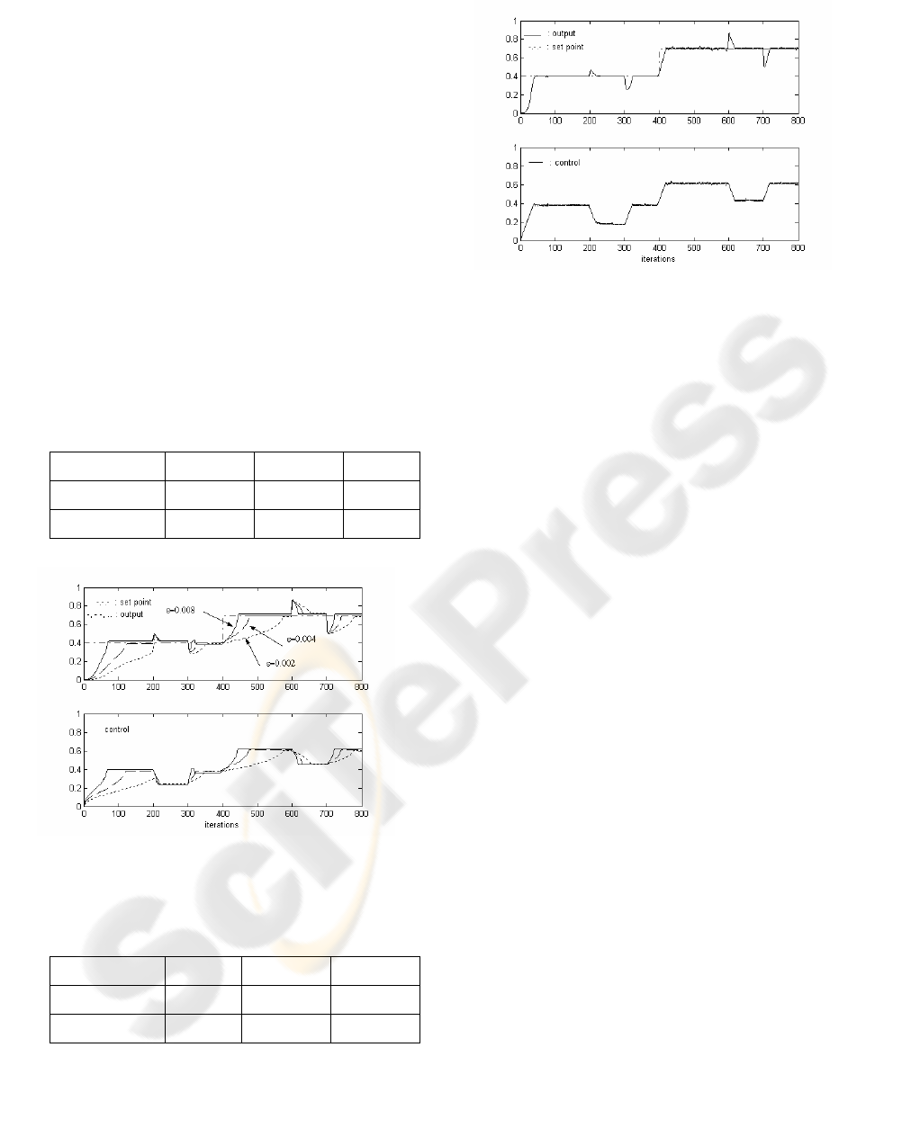
4.1 Ellipsoid Algorithm
The closed loop results shown in Figure 1 are
obtained for an initial ellipse characterized by a
center equals to 0.02 and
α
equals to 10. The
stopping criterion ε is chosen, respectively, equal to
0.002, 0.004 and 0.008. Load disruptions are added
to the output between the iterations (200, 300) and
(600, 700). The CPU time needs by the Ellipsoid
algorithm, at each simple time, is shown in table 1.
4.2 Genetic-Ellipsoid Algorithm
We have considered a genetic algorithm
characterized by a maximal number of generations
(maxgen) equals to 50; a crossover probability
P
c
=0.7; and a mutation probability P
m
=0.04. The
initial population is composed by 10 individuals
chosen arbitrary between 0 and 10. The centre of
the initial ellipse and the stopping criterion (ε) are
chosen respectively equal to 0.02 and 10
-5
. The
obtained closed loop results are shown in Figure 2.
The CPU time needs by the Genetic Ellipsoid
algorithm, at each simple time, is shown in table 2.
From figure 1, we notice that the closed loop
performances i.e. rise time, time needed to handle
load disruptions depend on the ellipsoid algorithm
parameters (A and ε). Indeed, the decreasing of the
stopping criterion ε leads to a slowly closed loop
dynamic. It’s clear from figure 2, that the proposed
method allows the designer to obtain a fast closed
loop dynamic with a small value of ε i.e. ε=10
-5
.
The Genetic Ellipsoid algorithm needs more time
ICINCO 2005 - INTELLIGENT CONTROL SYSTEMS AND OPTIMIZATION
290
than the EA. Consequently, it can be used only with
slow dynamical systems.
5 CONCLUSIONS
This paper was concerned with the constrained
nonlinear predictive control. A neural network
model is used to predict the system output over the
prediction horizon. Two methods are considered for
the non convex optimization. The first method is
based on the classical ellipsoid algorithm. The
second method combines genetic and ellipsoid
algorithms. Genetic algorithms are used to adjust
the EA parameters. The proposed algorithm allowed
us to overcome the problem of initialization the first
ellipsoid but increases the CPU time needed at each
simple time.
Table 1: CPU time of the ellipsoid algorithm
Value of A 10 10 10
ε 2 10
-3
4 10
-3
8 10
-3
CPU time (s) 9.77 10
-4
6.82 10
-4
5.5 10
-4
Figure 1: Set point, outputs and controls for different
values of ε (Ellipsoid algorithm)
Table 2: CPU time of the Genetic Ellipsoid algorithm
maxgen 25 50 100
ε 10
-5
10
-5
10
-5
CPU time (s) 1.0073 1.9641 3.7470
Figure 2: Set point, output and control (Genetic Ellipsoid
algorithm)
REFERENCES
Boyd S., El Ghaoui L., Feron E. and Balakrishnan V.
“Linear Matrix Inqualities in System and Control
Theory”, edition SIAM 1994
Clarke D. W., C. Mohtadi and P. S. Tuffs, “Generalized
predictive Control”. Part I and II, Automatica, Vol. 23,
No. 23, pp.137-160, 1987.
Goldberg D. E., "Genetic Algorithms in search,
optimization and machine learning", Addison-Wesley,
Massachusetts, 1991.
Hunt K. J., D. Sbarbaro, R. Zbikowski and P. J. Gawthrop,
"Neural networks for control systems - a survey",
Automatica, Vol. 28, No. 6, pp. 1083-1112, 1992.
Levin A. U. and K. S. Narendra, "Control of nonlinear
dynamical systems using neural networks”. Part II:
Observability, identification, and control, IEEE Trans.
Neural Networks, Vol. 7, No. 1, pp. 30-42, 1996.
Najim K., A. Rusnak, A. Meszaros and M. Fikar
"Constrained long-range predictive control based on
artificial neural networks", International Journal of
System Sciences, Vol. 28, No. 12, pp. 1211-1226,
1997.
Narendra K. S. and K. Parthasarathy, "Identification and
control of dynamical systems using neural networks",
IEEE Trans. Neural Networks, Vol. 1, No. 1, pp. 4-27,
1990.
Primoz P. and G. Igor, “Non linear model predictive
control of a cutting process” Neurocomputing, Vol.
43, pp. 107-126, 2002.
Saldanha R. R., R. H. C. Takahashi, J. A. Vasconcelos
and J. A. Ramirez, "Adaptive Deep-Cut Method in
Ellipsoidal Optimization for Electromagnetic Design",
IEEE Transactions on Magnetics, vol. 35, No. 3, pp.
1746-1749,1999.
Takahashi R. H. C., R. R. Saldanha, W. Dias-Filho and J.
A. Ramirez, "A New Constrained Ellipsoidal
Algorithm for Nonlinear Optimization With Equality
Constraints", IEEE Transactions on Magnetics, Vol.
39, No. 3, pp. 1289-1292, 2003.
GENETIC AND ELLIPSOID ALGORITHMS FOR NONLINEAR PREDICTIVE CONTROL
291
