
MOTION SEGMENTATION IN SEQUENTIAL IMAGES BASED ON
THE DIFFERENTIAL OPTICAL FLOW
Flavio de Barros Vidal
1
Victor Hugo Casanova Alcalde
2
Control and Computer Vision Laboratory
Electrical Engineering Department, University of Brasilia, 70910-900 Brasilia,DF - Brazil
Keywords:
Optical Flow, Motion Segmentation, Sequential Images.
Abstract:
This work deals with motion detection from image sequences. An algorithm to estimate the optical flow using
differential techniques is presented. Noise effects affecting motion detection were taken into account and
provisions to minimize it were implemented. The algorithm was developed within the Matlab environment
using mex-files to speed up calculations and it was applied to surveillance and urban traffic images. For the
considered cases, the results were quite satisfactory.
1 INTRODUCTION
Image motion segmentation is often coupled with
motion detection, where each region corresponds to
a particular motion model explaining the temporal
changes in that image region (Boult and Brown,
1991).
Several works describe techniques to separate or
extract the motion under certain hypothesis that as-
sures its applicability. Among the image motion ex-
tracting methodologies, we are interested in those
ones based upon optical flow. This technique has
been studied for application in areas such as biomedi-
cine, meteorology, visual inspection systems, process
control and real time urban traffic monitoring (Branca
et al., 1997) (Giachetti et al., 1998).
This work presents an approach to motion segmen-
tation in sequential images. Using the optical flow
concept, applying morphological transformations to
binary images, as well as, spatial processing the im-
age motion can be extracted. This procedure seems
to be independent on motion rigidity, on acquisition
conditions and on scene elements.
Initially the image segmentation for motion extrac-
tion is discussed (section 2). Section 3 deals with
the optical flow concept and its determination using
differential techniques, being the noise influence dis-
cussed. Section 4 describes the development and im-
plementation of the motion segmentation algorithm.
Finally, in section 5, results from the algorithm appli-
cation to indoors and outdoors images are presented.
2 IMAGE SEGMENTATION
Image segmentation has an important role on image
analysis and computer vision, finding the regions that
are associated to the objects in a given image. The
methodology is based upon low semantic content in-
formation, directly resulted from the neighborhood
proximities especially restricted, so that it is widely
classified as a low-level processing.
Segmentation algorithms are generally based on
one of two basic principles: discontinuity and simi-
larity (Gonzalez and Woods, 2000). In the first princi-
ple, the approach consists on image partitioning based
on rough changes in brightness. The main interests
here are the detection of isolated points, lines and
edges. In the second principle, the main approaches
are based on threshold levels and on growing, split-
ting and merging regions.
The choice of the segmentation technique depends
on the characteristics of each problem (Hendee and
Wells, 1997). For human beings it is easy to per-
ceive the movement of an object in reference to a
background. Trying to implement this procedure us-
ing computer-based artificial vision is a complex task.
The proposed algorithm applies image-processing
techniques and performs motion segmentation in an
efficient way for the examples here considered. It
shows to be independent of such factors as motion
rigidity and object shape.
94
de Barros Vidal F. and Hugo Casanova Alcalde V. (2005).
MOTION SEGMENTATION IN SEQUENTIAL IMAGES BASED ON THE DIFFERENTIAL OPTICAL FLOW.
In Proceedings of the Second International Conference on Informatics in Control, Automation and Robotics - Robotics and Automation, pages 94-100
DOI: 10.5220/0001183500940100
Copyright
c
SciTePress

3 OPTICAL FLOW
The optical flow approximates the image motion field
by representing the apparent motion of the image
brightness pattern on the image plane.
In determining the optical flow, two aspects must
be taken into account. One is related to the accuracy
level of data concerning motion direction and inten-
sity. The other aspect encompasses certain properties
related to the computational load required for optical
flow determination under minimal conditions of accu-
racy. The compromise between these aspects depends
on the situation and the expected results. The trade-
offs between efficiency and accuracy in optical flow
algorithms are discussed by (Liu et al., 1998).
The methods of determining the optical flow can be
divided (Barron et al., 1994) in: a) differential tech-
niques; b) region-based matching; c) energy-based
methods; and d) phase-based techniques. Initially we
considered the differential techniques. Among them,
one has a particular interest; it uses spatiotemporal
derivatives of the image brightness intensity (Horn
and Schunck, 1981). The optical flow can be obtained
from these variations. This technique assumes that
the motion is intrinsically coupled to image brightness
variations. It assumes as well that the scene illumina-
tion does not change; otherwise, the light changes will
influence the motion detection.
3.1 Horn & Schunck Differential
Method
According (Horn and Schunck, 1981) the optical flow
cannot be calculated at a point in the image inde-
pendently of neighboring points without introducing
additional constraints. This happens because the ve-
locity field at each image point has two components
while the change in brightness at that point due to mo-
tion yields only one constraint. Before describing the
method, certain conditions must be satisfied.
For convenience, it is assumed that the apparent ve-
locity of brightness patterns can be directly identified
with the movement of surfaces in the scene. This im-
plies that, according the object surface that moves, it
does not exist (or there is a little) brightness varia-
tion. This happens, for example, with objects of ra-
dial symmetry, low global contrast and high specular
reflectance level. It is further assumed that the inci-
dent illumination is uniform across the surface.
Denoting I(x, y, t) as the image brightness at time
t of the image point (x, y). During motion, it is as-
sumed that the brightness of a particular point is con-
stant, that means
dI (x, y, t)
dt
= 0 (1)
Expanding and rewriting the equation 1
I
x
u + I
y
v + I
t
= 0 (2)
where: I
x
, I
y
and I
t
represent partial derivatives of
brightness in x, y and t respectively; u and v are the
x− and y−velocity components.
Considering that, the brightness pattern can move
smoothly and independently of the rest of the scene,
there is a possibility to recover velocity information.
The partial derivatives of image brightness are esti-
mated from the discrete set of image brightness mea-
surements. To avoid problems caused by zero values
for the derivatives in the spatiotemporal directions,
the point of interest is located at the center of a cube
formed by eight measurements as shown in figure 1
(Horn and Schunck, 1981).
Figure 1: Estimating image partial derivates
Each of the partial derivatives is estimated as the
average of the four first differences taken over adja-
cent measurements
I
x
≈
1
4
{I
i,j+1,k
− I
i,j,k
+ I
i+1,j+1,k
− I
i+1,j,k
+
I
i,j+1,k+1
− I
i,j,k+1
+ I
i+1,j+1,k+1
− I
i+1,j,k+1
}
I
y
≈
1
4
{I
i+1,j,k
− I
i,j,k
+ I
i+1,j+1,k
− I
i,j+1,k
+
I
i+1,j,k+1
− I
i,j,k+1
+ I
i+1,j+1,k+1
− I
i,j+1,k+1
}
I
t
≈
1
4
{I
i,j,k+1
− I
i,j,k
+ I
i+1,j,k+1
− I
i+1,j,k
+
I
i,j+1,k+1
− I
i,j+1,k
+ I
i+1,j+1,k+1
− I
i+1,j+1,k
}
(3)
The additional constraint for the velocity calcula-
tion results from the assumption of smoothness of the
velocity field. The solution to the optical flow prob-
lem consists therefore in: a) minimize equation 4; and
b) minimize the smoothness measurement of the ve-
locity field. Equation (5) is a measure of the departure
from smoothness in the velocity field. For minimiza-
tion two errors are defined
ξ
b
= I
x
u + I
y
v + I
t
(4)
and
MOTION SEGMENTATION IN SEQUENTIAL IMAGES BASED ON THE DIFFERENTIAL OPTICAL FLOW
95
ξ
2
c
=
∂u
∂x
2
+
∂u
∂y
2
+
∂v
∂x
2
+
∂y
∂x
2
(5)
The total error to be minimized will be
ξ
2
=
ZZ
α
2
ξ
2
c
+ ξ
2
b
dxdy (6)
A weighting factor α
2
is introduced to associate the
error magnitude with quantization errors and noise.
Using the Gauss-Seidel iterative method (Hilde-
brand, 1974) to minimize equation (6) one obtains u
and v velocity components. The estimated values for
u
k+1
and v
k+1
are obtained from
u
k+1
=
u
k
−
I
x
I
x
u
k
+ I
y
v
k
+ I
t
α
2
+ I
2
x
+ I
2
y
(7)
v
k+1
=
v
k
−
I
y
I
x
u
k
+ I
y
v
k
+ I
t
α
2
+ I
2
x
+ I
2
y
(8)
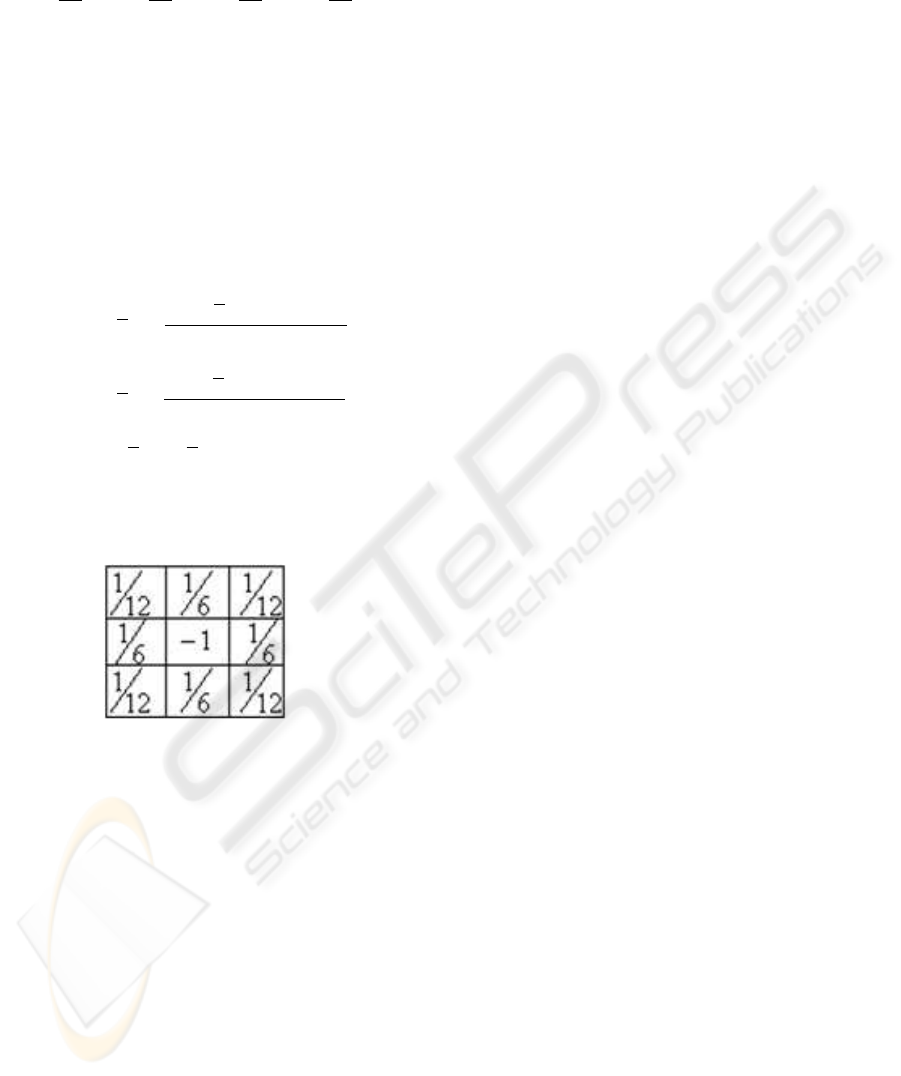
In equation (8)
u
k
and u
k
are the average velocities
estimated from the Laplacian of the brightness pattern
in iteration k, in which the neighboring pixels values
are weighted with the mask shown in figure 2.
Figure 2: Laplacian estimation mask
Figure 3 shows the image sequence from: a) sur-
veillance video camera; b) urban traffic monitoring
camera; and c) robot soccer game (synthetic images).
Figure 4 shows the calculated optical flow, sketched
as directional arrows, for the examples in Figure 3.
3.2 Influence of the α weighting
factor
In equations (7) and (8), the weighting factor α
2
rep-
resents a threshold effect upon the obtained velocity
field. By varying this weighting factor, the sensitiv-
ity level of the motion to undesirable data can be ad-
justed. This effect was applied in the implementation
of the algorithm for motion segmentation. Figure 5
shows the influence of the weighting factor in motion
segmentation.
4 MOTION SEGMENTATION
ALGORITHM
Most of the image segmentation methods demand a
previous knowledge of the model in order to produce
reasonable results. The algorithm here presented uses
information that is not dependent on the kind of mo-
tion. Initially the time and space information are de-
coupled. After this, the problem consists on segment-
ing the components of the obtained motion map.
4.1 Algorithm Overview
The algorithm consists of three fundamental sections,
as shown in figure 6. The first section of the algorithm
is the extraction of a map that contains information
related to the scene motion intensity.
The motion map is obtained adjusting the α weight-
ing factor during the optical flow calculation. This
adjustment affects the accuracy and intensity levels
of the resulting map.
The second section of the algorithm consists of a
sequence of post-processing techniques to analyze the
obtained map as an image by itself.
The procedures in the post-processing step (Figure
7) are applied sequentially:
a) Noise filtering - for eliminating noises from the
motion map computation. A Wiener low-pass
adaptive filter was applied. It uses stochastic in-
formation related to the pixel neighborhood, yield-
ing then satisfactory results (Gonzalez and Woods,
2000).
b) Binarization - for image binarization an optimum
threshold is obtained from the motion map his-
togram; and
c) Morphological filtering - to obtain the contour of
the segmented element. The structure element used
is adjusted according the size of the object to be
segmented.
The third section of the algorithm implements the
interpretation of the obtained segmentation. It ex-
tracts the contour of the region that moved in the im-
age.
5 RESULTS
The motion segmentation algorithm was applied to
the surveillance, urban traffic and robot soccer scenes
and the results in figures 8, 9 and 10 respectively. All
the sequences were obtained by using a fixed camera,
with 320 x 240 pixels of spatial resolution and with a
1 frame/sec sample image rate.
ICINCO 2005 - ROBOTICS AND AUTOMATION
96

(a)
(b)
(c)
Figure 3: Applications: (a) Surveillance camera sequence; (b) Urban traffic sequence; (c) Robot soccer game (synthetic)
sequence.
The algorithm was developed within the Matlab en-
vironment. To speed up data processing, sub-routines
in C language for critical procedures were written and
incorporated as mex-files (a Matlab feature).
Case 1: Surveillance Camera - Figure 8 illustrates
the motion of a single person through an environ-
ment surrounded by many objects. Moreover, there
are some regions with a high degree of ambiguities.
The influence of ambiguities is higher on the other
methods of determining the optical flow than the ones
that use differential techniques (Barron et al., 1994).
Case 2: Urban Traffic Monitoring - Figure 9
shows many objects moving along different direc-
tions. There are then situations with shape change
(perspective), occlusions and ambiguities.
Case 3: Robot Soccer Game - Figure 10 shows
the robot players performing translation and rotation
movements to implement a soccer game. For syn-
thetic images, the algorithm performs more efficiently
due the reduced noise and quantization interference
over the motion segmentation.
For the cases studied, the algorithm segmented the
objects and the moving objects were tracked success-
fully. For the cases studied, the values of a factor and
of the structuring element were adjusted for the best
results. The adjusted values are shown in table 1.
The errors shown in table 1 were calculated from a
comparison of the moving object area to the area of
the region bounded by the algorithm.
MOTION SEGMENTATION IN SEQUENTIAL IMAGES BASED ON THE DIFFERENTIAL OPTICAL FLOW
97

(a) (b)
(c)
Figure 4: Optical flows using Horn & Schunck method for the cases in Fig. 3. (a) Surveillance camera sequence; (b) Urban
traffic sequence; and (c) Robot soccer game sequence.
(a) (b)
Figure 5: Variation of α factor for the urban traffic sequence, (a) α = 10; (b) α = 100
ICINCO 2005 - ROBOTICS AND AUTOMATION
98

Figure 6: Algorithm main loop
Table 1: Setup Algorithm Parameters
Sequence α
Structuring
Element Size
Error
Estimative
Surveillance
Camera
1 18 ∼ 10.5%
Urban Traffic 75 7 ∼ 8.3%
Robot Soccer 10 12 ∼ 5.1%
6 CONCLUSIONS
This works presents an algorithm for segmenting im-
age motion by determining an optical flow calculated
through differential methods. The determination of
the optical flow allows varying a weighting factor,
which allows adjusting the sensitivity level of the mo-
tion to undesirable data.
Within the post-processing stage of the algorithm,
a morphological filtering step allows adjusting the
structuring element according to a given situation. As
shown in the results, the limit region motion was suc-
cessfully tracked, with acceptable errors. The algo-
rithm does not use parametrical methods; it needs
not pre-calibration or additional image improvements,
showing then some robustness to motion complexity.
An upgrade to the algorithm would be the inclusion
of the feature of an auto-adjustable structuring ele-
ment that uses information from the motion map. Fur-
ther work would be the conception of a hybrid image-
tracking algorithm to estimate moving regions by dif-
ferential methods and their tracking using region-
based matching techniques. This approach could re-
duce the computational effort and processing time de-
manded by these matching techniques, which search
Figure 7: Description post-processing step
Figure 8: Surveillance sequence segmented
throughout the whole image. Performing the segmen-
tation previously, the search is restricted only to those
regions of interest.
REFERENCES
Barron, J. L., Fleet, D. J., and Beauchemin, S. S. (1994).
Performance of optical flow techniques. In Inter-
national Journal of Computer Vision, number 12:1,
pages 43–77.
Boult, T. E. and Brown, L. G. (1991). Factorization-based
segmentation of motion. In IEEE Workshop on Visual
Motion, pages 179–186. IEEE.
Branca, A., Cicirelli, G., Stella, E., and Distante, A.
(1997). Mobile vehicle’s egomotion estimation from
MOTION SEGMENTATION IN SEQUENTIAL IMAGES BASED ON THE DIFFERENTIAL OPTICAL FLOW
99

time varying image sequences. In International Con-
ference of Robotics and Automation, pages 1886–
1891.
Giachetti, A., Campani, M., and Torre, V. (1998). The use of
optical flow for road navigation. In IEEE Transactions
on Robotics and Automation, number 14, pages 34–
48. IEEE.
Gonzalez, R. C. and Woods, R. E. (2000). Processamento
de Imagens Digitais.
Hendee, W. R. and Wells, P. N. T. (1997). The perception
of Visual Information. Second edition edition.
Hildebrand, F. B. (1974). Introduction to Numerical Analy-
sis.
Horn, B. K. P. and Schunck, B. G. (1981). Determining op-
tical flow. In Artificial Intelligence, number 17, pages
185–204.
Liu, H., Hong, T., Herman, M., Camus, T., and Chellappa,
R. (1998). Accuracy vs efficiency trade-offs in opti-
cal flow algorithms. In Computer Vision and Image
Understanding, number 72:3, pages 271–286.
Figure 9: Urban Traffic sequence segmented
Figure 10: Robot soccer sequence segmented
ICINCO 2005 - ROBOTICS AND AUTOMATION
100
