MOBILE ROBOT PREDICTIVE TRAJECTORY TRACKING
Martin Seyr
Vienna University of Technology, Institute of Mechanics and Mechatronics
Gusshausstrasse 27-29, A-1040 Wien
Stefan Jakubek
Vienna University of Technology, Institute of Mechanics and Mechatronics
Gusshausstrasse 27-29, A-1040 Wien
Keywords:
mobile robot, trajectory tracking, nonholonomic system, nonlinear predictive control.
Abstract:
For a two-wheeled differentially driven mobile robot a trajectory tracking concept is developed. A trajectory
is a time-indexed path in the plane, i.e. in the three-dimensional configuration space consisting of position and
orientation. Due to the nonholonomic nature of a rolling wheel, the system cannot be stabilized by a contin-
uous time-invariant feedback or by feedback linearization. A novel approach taken in this paper to solve the
nonholonomic control problem consists of nonlinear predictive control in conjunction with linear state space
control with integration of the control error. Based on a Gauss-Newton algorithm, predicted future position
errors are minimized by numerical computation of an optimal sequence of control inputs using prespecified
shape functions.
1 INTRODUCTION
The basic task in mobile robot motion control is to ac-
curately follow a given trajectory. The error between
the present posture x(t) = [x(t) y(t) ϕ(t)]
T
and the
reference trajectory is to be minimized.
Considerable research has been done on trajectory
tracking control of the unicycle-type mobile robot. Its
kinematics are a classical example of a nonholonomic
nonlinear control system, the nonholonomic integra-
tor (NHI), in somewhat different form also known as
Brockett- or Heisenberg-system.
It was first shown by (Brockett, 1983), that this sys-
tem cannot be stabilized by continuous, time-invariant
feedback, although it is controllable in a nonlinear
sense.
Furthermore, it can be shown using a methodology
by (Isidori, 1989), that the NHI cannot be feedback-
linearized.
Therefore, various control concepts trying to cir-
cumvent the aforementioned limitations have been
presented in recent years. Among the major groups
of approaches are sliding-mode control, e.g. (Bloch
and Drakunov, 1994), time-varying feedback laws,
e.g. (Samson, 1995), hybrid control laws, e.g. (Hes-
panha and Morse, 1996) and dynamic feedback lin-
earization, e.g. (Oriolo et al., 2002).
None of the mentioned publications deal with the
problem of non-zero side-slip angle. Some do not
take the dynamics of the system into account, they
are only concerned with its kinematics.
A drawback inherent to many of the concepts
present in the literature is a singularity in the con-
trol law occurring at zero velocity, e.g. (Oriolo et al.,
2002).
In the present paper, a novel approach is presented
employing numerical optimization of open loop con-
trol rather than any explicit feedback control law.
Therefore, the aforementioned restrictions do not ap-
ply here.
This concept is made possible by the robot’s out-
standing on-board calculation capacity provided by a
microcontroller and a digital signal processor.
2 THE PLANT: AN
AUTONOMOUS
TWO-WHEELED MOBILE
ROBOT
The robot, Fig. 1, has two wheels with rubber tires
and two felt shoes, one at the front and one at the rear
to stabilize it around the pitch axis. It fits into a cuboid
with a 0.075m square footprint. The two wheels are
supported by ball bearings and powered by two indi-
112
Seyr M. and Jakubek S. (2005).
MOBILE ROBOT PREDICTIVE TRAJECTORY TRACKING.
In Proceedings of the Second International Conference on Informatics in Control, Automation and Robotics - Robotics and Automation, pages 112-119
DOI: 10.5220/0001184001120119
Copyright
c
 SciTePress

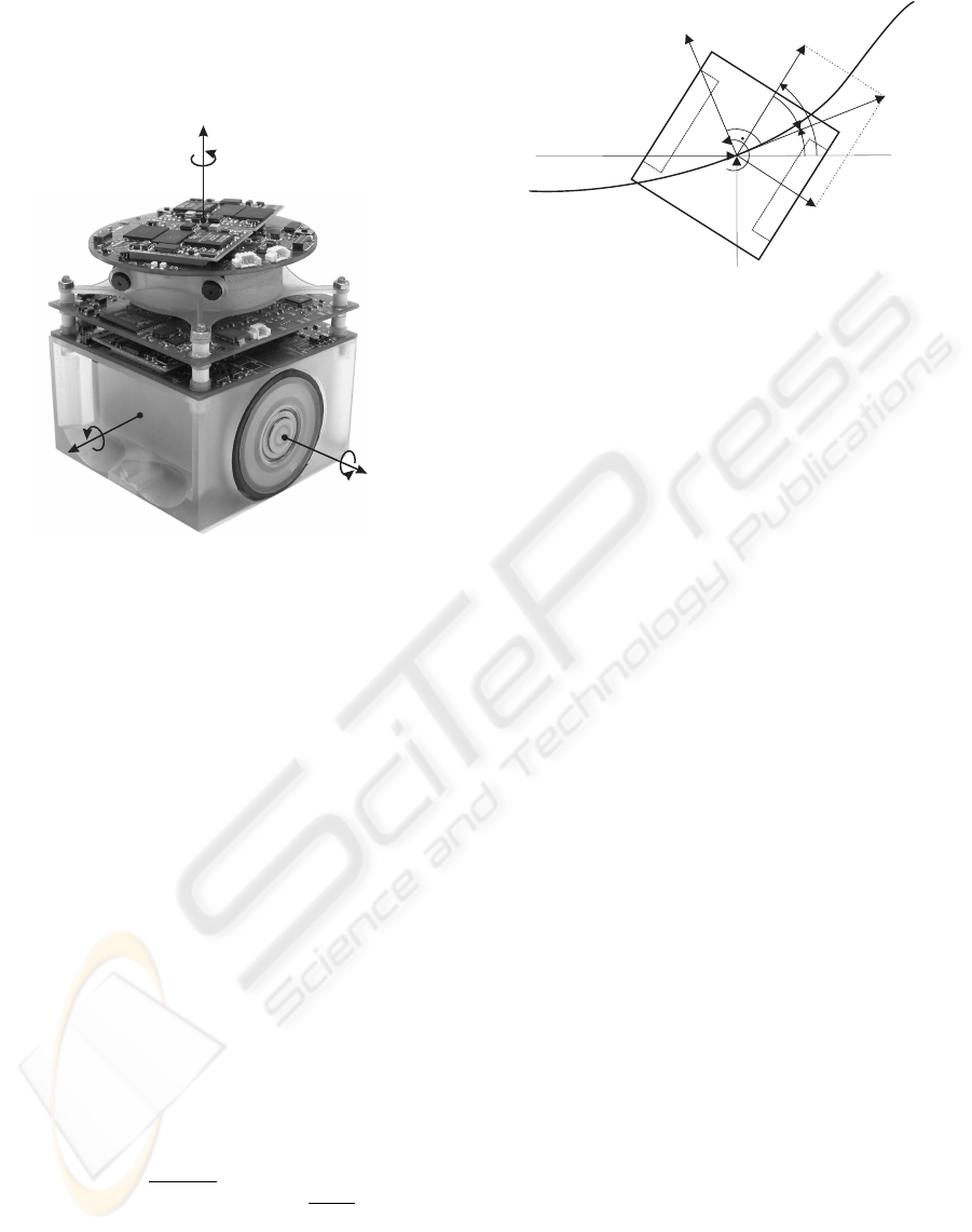
vidual DC-motors. A microcontroller produces two
pulse-width modulated (PWM) constant voltage sig-
nals, which are amplified by a dual full bridge driver.
The amplified signals drive the two DC-motors.
Yaw-axis
Pitch-axis
Roll-axis
x
y
z
Figure 1: Autonomous mini-robot Tinyphoon,
http://www.tinyphoon.com
Nonlinearities originate from variable switching
times and dead zones in the amplifier circuit, fric-
tion characteristics of bearings and gearboxes and
the wheel slip dynamics. The kinematics of a two-
wheeled mobile robot are equivalent to those of a sin-
gle rolling wheel. Therefore, this system is often re-
ferred to as the unicycle-type mobile robot.
The dynamics of the entire system will be partitioned
into those of the path velocity and yaw angular ve-
locity, which can be linearized to form a two-input-
two-output linear state space system, and the nonlin-
ear nonholonomic kinematics.
2.1 Velocity dynamics
To obtain a linearization of the velocity dynamics, a
number of simplifications are made:
1. The slip-dynamics are omitted,
2. the side-slip velocity v
n
and the tangential veloc-
ity v
t
are combined to an effective track speed v,
Fig. 2,
v =
q
v
2
t
+ v
2
n
signv
t
=
v
t
cos α
, (1)
3. the motor characteristic is linearized using least
squares with a bilinear regressor function.
The result is a linear continuous-time state space
system with state vector v := [v ω]
T
and input vector
u := [r
PWM,r
r
PWM,l
]
T
,
a
v
v
n
v
t
ω
α
x
y
θ
ϕ
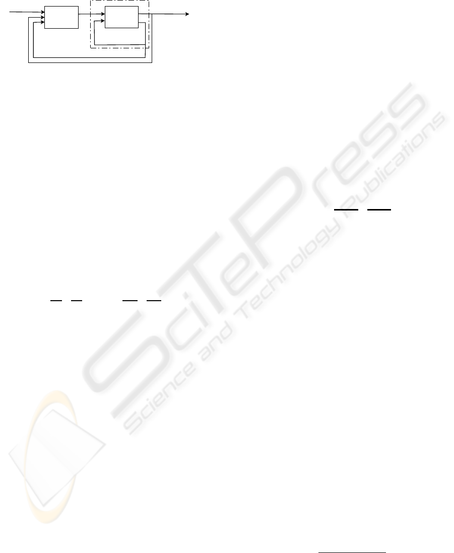
Figure 2: Kinematics of a two-wheeled mobile robot under
consideration of side slip and tangential wheel slip
˙
v =

a 0
0 c

v +

b b
d −d

u, (2)
where the parameters have been collected to form
the constants a, b, c and d, and r
PWM,r
and r
PWM,l
denote the PWM-duty cycles of the right and left mo-
tor input voltages.
2.2 Kinematics
The kinematics of the unicycle-type mobile robot are
given by
˙x = v cos(ϕ + α)
˙y = v sin(ϕ + α)
˙ϕ = ω, (3)
where x and y denote the inertial coordinates and
ϕ denotes the inertial attitude angle of the robot.
From Fig. 2 it can be seen that
θ = ϕ + α, (4)
where θ denotes the angle of the tangent to the ac-
tual path.
3 CONTROL CONCEPT
Since the velocity dynamics and the kinematics can
be solved consecutively (i.e. the result of the veloc-
ity dynamics serves as input into the kinematics, but
there is no influence of the positions on the veloci-
ties), the application of a cascading control scheme is
straightforward.
The chosen scheme employs a linear state feedback
law with integration of the velocity errors to control
the velocities v, in the following referred to as the
inner loop, and a nonlinear predictive controller us-
ing the closed loop dynamics of the inner loop in the
MOBILE ROBOT PREDICTIVE TRAJECTORY TRACKING
113

prediction of the positions x (in the following: outer
loop), Fig. 3.
Predictor
State-space
x
ref
(k . . . k + h
p
)
v
ref
(k)
x(k)
v (k)
Closed loop dynamics
Figure 3: Cascaded control scheme, h
p
denotes the predic-
tion horizon
4 CONTROL OF THE INNER
LOOP
4.1 Discretization
First, the continuous-time state space representation
of the robot’s dynamics is discretized assuming that
a zero-order hold acts at the input. Theoretical back-
ground can be found e.g. in (Isermann, 1987).
The system (2) is then written as
v(k +1) =

p 0
0 r

|
{z }
A
v(k)+

q q
s −s

|
{z }
B
u(k), (5)
where p, q, r, s are real-valued constants and k de-
notes the integer sampling instants.
4.2 Extended system
The control algorithm’s calculation time must be ex-
pected to consume a considerable portion of the sam-
pling interval, therefore the common assumption, that
the output of a control algorithm is available instanta-
neously, does not hold.
On the contrary, it must be assumed, that the output of
the controller can only be applied at the beginning of
the next sampling interval. Basically, this would lead
to a control law of the form
u(k) = f(v(k − 1), v
ref
(k − 1)), (6)
i.e. a one-step deadtime in the control law itself
unless a prediction for v(k) is used.
Therefore, the order of the system is deliberately
increased by using past values as additional states, so
as to be able to use v(k − 1) in the control law for
u(k).
In the outer loop, a prediction for the future
velocities is calculated anyway (indicated with aˆ).
Practical tests show, however, that it is still advisable
to use the extended system for controller design,
since a feedback law based entirely on predicted
values tends to destabilize quickly.
After introducing the integrated control errors q as
additional states, the extended system is written as
"
v(k + 1)
v(k)
q(k)
#
=
"
A 0 0
I 0 0
0 −I I
#"
ˆ
v(k)
v(k − 1)
q(k − 1)
#
+
+
"
B
0
0
#
u(k) +
"
0
0
I
#
v
ref
(k − 1). (7)
The static state feedback control law has the form
u(k) = K
|{z}
2×6
"
ˆ
e(k)
e(k − 1)
−q(k − 1)
#
|
{z }
6×1
, (8)
where K denotes the feedback gain matrix, calcu-
lated using standard pole assignment procedures.
5 CONTROL OF THE OUTER
LOOP
The principle of nonlinear predictive control using a
Gauss-Newton-optimization algorithm is taken from
(Norgaard et al., 1999), where this procedure is ap-
plied to SISO-systems (single-input-single-output),
which are dynamically modeled by recurrent multi-
layer perceptron networks (MLP).
The algorithm is adapted to use a nonlinear MIMO-
state space representation instead of the MLP-
network.
A similar procedure for a MIMO-neural network was
used in (Seyr and Jakubek, 2005).
5.1 Discretization of the kinematic
model
First, the continuous time nonlinear state space sys-
tem (3) is discretized using a simple forwards differ-
ence approximation (explicit Euler) for the first order
derivatives,
˙x(k) =
x(k + 1) − x(k)
T
s
,
analogously for y and ϕ.
Then the system (3) can be written as
ICINCO 2005 - ROBOTICS AND AUTOMATION
114

x(k + 1) = T
s
v(k) cos[ϕ(k) + α(k)] + x(k)
y(k + 1) = T
s
v(k) sin[ϕ(k) + α(k)] + y(k)
ϕ(k + 1) = T
s
ω(k) + ϕ(k). (9)
5.2 Cost function
Predictive control is based on the minimization of
a scalar quadratic cost function containing predicted
future position errors P and future control variables
V
ref
during every sampling interval, here denoted for
a system with three outputs (x := [x y ϕ]
T
) and two
control variables (v
ref
:= [v
ref
ω
ref
]
T
). For the two
control variables, shape functions are chosen. The
shape of the future control variables is then adjusted
using two parameters each. The cost as a function of
the form-parameters c reads
V =
1
2h
p
P
T
LP +
1
2
c
T
Rc, (10)
where
P =














x
ref
(k + 3) − x(k + 3)
x
ref
(k + 4) − x(k + 4)
.
.
.
y
ref
(k + 3) − y(k + 3)
.
.
.
y
ref
(k + h
p
) − y(k + h
p
)
.
.
.
ϕ
ref
(k + h
p
) − ϕ(k + h
p
)














.
The structure of the shape functions for v
ref
and
ω
ref
is identical and given by
v, ω
ref
(k) = c
1,3
+ c
2,4
(1 − exp(−κkT
s
))
|
{z }
f(k)
, (11)
where the curvature of the shape function can be
adjusted by the form factor κ: from almost linear
(κ <<) to steep at the beginning and flat at the
end (κ >>), which influences the bandwidth of the
system.
Additionally, the second part f (k) is scaled to ensure
comparable influence of c
2,4
when using different
values for κ.
• The cost function V is evaluated and minimized
during each sampling interval.
• Future reference values x
ref
up to the prediction
horizon h
p
must be known.
• The form-parameters c, shaping the v
ref
up to the
control horizon h
u
(here: h
u
= h
p
− 2), are opti-
mized using (10).
• The weight matrices L ∈ IR
3(h
p
−2)×3(h
p
−2)
and
R ∈ IR
4×4
determine to what extent the future con-
trol variables and the future control errors are con-
sidered.
From measurement data, the current posture
[x(k) y(k) ϕ(k)]
T
) and velocities [v(k) ω(k)]
T
are
calculated.
Using the first and the last line of the closed loop state
space representation of the inner loop
v(k + 1) =
= [
A − BK
1
−BK
2
−BK
I
]
"
v(k)
v(k − 1)
q(k − 1)
#
+
+ [
BK
1
BK
2
]

v
ref
(k)
v
ref
(k − 1)

,
and
q(k) = [
0 −I I
]
"
v(k)
v(k − 1)
q(k − 1)
#
+
+ [
0 I
]

v
ref
(k)
v
ref
(k − 1)

, (12)
estimated future velocities and velocity error
integrals can be calculated recursively.
Next, the predicted positions are calculated by (9).
Therefore, the current side-slip angle α(k) has to be
determined. The current position x
k
= [x
k
y
k
] and
the last two positions x
k−1
and x
k−2
are transformed
to local coordinates, Fig. 4,
x
k−i,loc
=

cos θ
k−1
sin θ
k−1
− sin θ
k−1
cos θ
k−1

[x
k−i
−x
k−1
],
(13)
where i ∈ [0 1 2]. Next, the parameters of a Spline-
approximation of x(k − i) and y(k − i) are calculated
using a quadratic regressor [1 t t
2
] and dimension-
less time t ∈ [0; 2] according to
"
a
x,0
a
x,1
a
x,2
#
=
"
1 0 0
1 1 1
1 2 4
#
−1
"
x
k−2
x
k−1
x
k
#
. (14)
The increment of the path angle ∆θ is calcu-
lated by evaluating the derivatives of the Spline-
approximations at time t = 2,
∆θ
k
= atan
dy
dx
= atan
dx/dt
dy/dt
= atan
a
y , 1
+ 4a
y , 2
a
x,1
+ 4a
x,2
.
(15)
Finally, the actual side-slip angle is given by
MOBILE ROBOT PREDICTIVE TRAJECTORY TRACKING
115

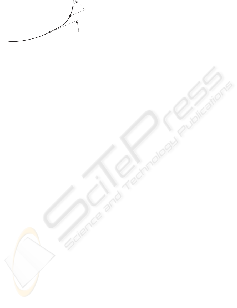
∆θ
k
θ
k−1
x
k
x
k−1
x
k−2
t = 0
t = 1
t = 2
Figure 4: Estimation of the current path angle θ
k
α
k
= θ
k
− ϕ
k
= θ
k−1
+ ∆θ
k
− ϕ
k
. (16)
The incremental calculation of the path angle has
the decisive advantage that possible transgressions
of the interval [−π; π] do not have to be accounted for.
Naturally, no meaningful results for the path angle
are obtained for zero track speed v. Therefore,
the path angle is set equal to the attitude angle for
small values of v below a certain margin, followed
by a short region of linear interpolation to ensure
continuity and finally taken full beyond another
threshold of v.
When using possibly noise corrupted measurement
data, the estimation can also be performed using a
greater number of previous positions, then employing
a least squares estimator.
To control the inertial attitude angle, the current
side-slip α is subtracted from the reference path angle
θ
ref
, thus obtaining a feasible reference attitude ϕ
ref
.
After the computation of an initial estimate of the
future positions x, under the assumption that the side-
slip angle α remains constant over the prediction hori-
zon, the position errors p = x
ref
− x are calculated
and concatenated in P .
5.3 Minimization
The position errors are now approximated in a first
order Taylor series expansion,
P
.
= P
0
+
∂P
∂V
ref
∂V
ref
∂c
c =
P
0
−
∂X
∂V
ref
∂V
ref
∂c
c := P
0
− D
X
D
V
c. (17)
The matrix D
X
∈ IR
3(h
p
−2)×2(h
p
−2)
can be writ-
ten as
D
X
=











∂x(k + 2 + i)
∂v
ref
(k + j)
∂x(k + 2 + i)
∂ω
ref
(k + j)
∂y(k + 2 + i)
∂v
ref
(k + j)
∂y(k + 2 + i)
∂ω
ref
(k + j)
∂ϕ(k + 2 + i)
∂v
ref
(k + j)
∂ϕ(k + 2 + i)
∂ω
ref
(k + j)











,
(18)
with i, j ∈ [1; h
p
− 2], and D
V
∈ IR
2(h
p
−2)×4
reads
D
V
=









1 f(1) 0 0
1 f(2) 0 0
.
.
.
.
.
.
0 0 1 f(1)
0 0 1 f(2)
.
.
.
.
.
.









(19)
The total derivatives of the positions with respect
to the reference velocities are calculated recursively.
The total derivatives of the velocities V and the ve-
locity error integrals Q (where Q is the vector of ve-
locity error integrals concatenated of q in the exact
same way as P ) with respect to the reference veloci-
ties V
ref
are needed during the calculation of the total
derivatives of the positions X.
The dependencies are
x(k + 2 + i) = f
1
(x(k + 1 + i), v(k + 1 + i))
v(k+1+i) = f
2
(v(k+i), v(k− 1+i), q(k − 1+i),
v
ref
(k + i), v
ref
(k − 1 + i))
q(k+i) = f
3
(v(k−1+i), q(k−1+i), v
ref
(k−1+i)),
where the functions f
1
through f
3
are given by
(9) and (12).
The cost function (10) now reads
V (c) =
1
2
c
T
Rc+ (20)
+
1
2h
p
(P
0
− D
X
D
V
c)
T
L(P
0
− D
X
D
V
c).
To ensure closed loop stability of the inertial angle,
which proved to be critical during testing, a terminal
constraint for the inertial angle is introduced, (Mayne
et al., 2000) and references therein.
To fulfill the terminal constraint, an additional term
with a Lagrange-multiplier is added to the cost func-
tion. The additional term reads
ICINCO 2005 - ROBOTICS AND AUTOMATION
116

λ (ϕ(k + h
p
; c) − ϕ
ref
(k + h
p
))
.
=
λ (ϕ
0
(k + h
p
) − ϕ
ref
(k + h
p
))
|
{z }
∆ϕ
end
+λD
ϕ
c, (21)
where the 1 × 4 row vector D
ϕ
is the last
row of D
X
D
V
, i.e. the derivatives of ϕ(k + h
p
)
with respect to the form-parameters, and λ is the
Lagrange-multiplier. The second term in (21) is
a first order Taylor approximation of an otherwise
nonlinear constraint.
Minimization under fulfilment of the terminal
constraint is then obtained by differentiating with
respect to c and λ and equating the derivative with
zero.
After some algebraic manipulations the linear sys-
tem of equations with dimension 5
1
h
p
D
T
V
D
(ν)T
X
LD
(ν)
X
D
V
+ R D
(ν)T
ϕ
D
(ν)
ϕ
0
c
(ν)
λ
(ν)
=
=
−
1
h
p
D
T
V
D
(ν)T
X
LP
(ν)
0
∆ϕ
(ν)
end
, (22)
written with index ν for the ν-th cycle of the
iteration, is obtained.
With the calculated form-parameters c, the future
reference velocities V
ref
are updated.
v, ω
(ν+1)
ref
(k + 1 + i) = (23)
= v, ω
(ν)
ref
(k + 1 + i) + c
(ν)
1,3
+ c
(ν)
2,4
f(i)
Then, the updated prediction of the position errors
P
(ν+1)
0
and the matrix of derivatives D
(ν+1)
X
at the
new predicted positions are calculated.
After a specified number of iterations, the algorithm
terminates. Usually, a few cycles are sufficient to
achieve convergence.
The weight matrices L and R, the prediction
horizon h
p
, the form factor κ, the sampling time
T
s
and the number of iterations performed are the
design parameters and substantially influence the
performance of the system.
The optimization of a few form-parameters instead
of an entire reference velocity sequence reduces the
calculation time significantly, since only a 5 × 5-
system of equations has to be solved every iteration.
Moreover, the solution is more robust and the sys-
tem’s bandwidth can be adapted selectively.
Prediction and optimization using the estimated
side-slip angle α leads in some situations to unsta-
ble oscillatory behaviour of the side-slip angle during
tracking of stationary curves, while the reference po-
sitions are matched with high accuracy.
On the other hand, when omitting the side-slip angle
in the optimization, position precision is deteriorated.
The controller then attempts to match the attitude an-
gle of the robot with the reference path angle, which
makes it physically impossible to keep the reference
position at large side-accelerations, because the side
force is generated by the side-slip.
Therefore, a compromise between stability and accu-
racy is sought by reducing the estimated side-slip an-
gle α by a relaxation factor µ. A value of about 0.9
to 0.95 provides stability throughout the entire feasi-
ble 2-dimensional velocity-curvature domain for sta-
tionary curves, while keeping position precision at a
reasonable level.
5.4 Application of the control law of
the inner loop
The velocity error
ˆ
e(k + 1) can now be calculated, as
mentioned before. The velocity error integral q(k) is
known from the first step of the prediction.
Therefore, the control law of the inner loop (8), writ-
ten for time k + 1
u(k + 1) = K
"
ˆ
e(k + 1)
e(k)
−q(k)
#
(24)
is now used to compute the PWM-input signals to
the DC-motors, which are applied at the end of the
current sampling interval, i.e. at time k + 1.
This means that the algorithm can consume the en-
tire sampling interval to calculate the output without
any negative effect on the control performance. The
calculation time is thus effectively compensated for,
provided it does not exceed the duration of one sam-
pling interval.
6 RESULTS
To test the tracking algorithm, simulations are carried
out using the nonlinear model.
Changing ground conditions are modeled via low fre-
quency noise or step changes acting on the respective
parameters of the nonlinear model.
The effect of possible modeling inaccuracies is simu-
lated by simply modifying various parameters used in
controller design.
To show the ability of the system to cope with
changing ground conditions, a stationary curve (i.e.
a circle) with a moderate centripetal acceleration
MOBILE ROBOT PREDICTIVE TRAJECTORY TRACKING
117

of 2.9ms
−2
, starting and ending with a sinusoidal
curvature-over-arclength profile and linear acceler-
ation and deceleration of the track speed, Fig. 5, is
used as reference trajectory, fed to the control algo-
rithm in terms of reference x-, y- and θ-sequences.
0 1 2 3 4 5 6 7
−0.5
0
0.5
1
1.5
2
2.5
t [s]
Velocity v, curvature ρ, [ms
−1
], [m
−1
]
ρ
v
Figure 5: Velocity and curvature profile used to generate the
reference trajectory
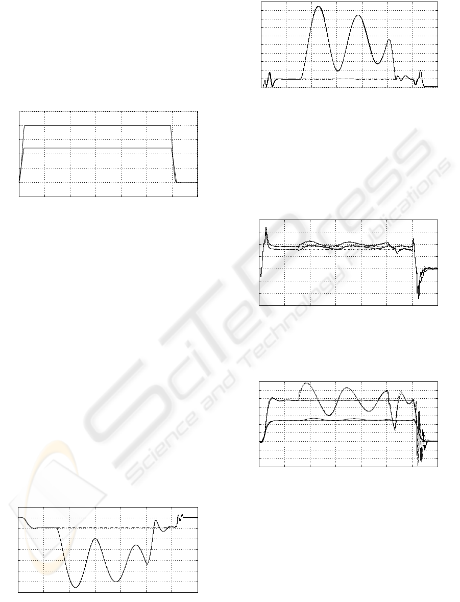
After 1.5s, the ground friction drops to 70% of
the initial value and returns to 100% after 5s. The
absolute of the side-slip angle increases drastically to
peak values near 35
◦
, Fig. 6. Stability is maintained,
the position error, however, increases almost pro-
portionally with the absolute of the side-slip angle,
reaching peak values of below 5cm, Fig. 7. Low
frequency damped oscillations of the side-slip angle
can be observed.
For comparison, the plots are underlayed with the
results for the same trajectory without disturbances.
0 1 2 3 4 5 6 7
−35
−30
−25
−20
−15
−10
−5
0
5
t [s]
Side slip α, [
◦
]
Figure 6: Side-slip angle with and without disturbance
(dashed)
0 1 2 3 4 5 6 7
0
0.005
0.01
0.015
0.02
0.025
0.03
0.035
0.04
0.045
0.05
t [s]
Position error, [m]
Figure 7: Absolute position error with and without distur-
bance (dashed)
The corresponding input signals r
PWM,r
and
r
PWM,l
are depicted in Fig. 8 and the calculated ref-
erence velocities v
ref
and ω
ref
and the true velocities
v and ω are displayed in Fig. 9.
0 1 2 3 4 5 6 7
−0.6
−0.4
−0.2
0
0.2
0.4
0.6
0.8
t [s]
PWM-signal r
PWM,r
and r
PWM,l
, [-]
right
left
Figure 8: Right and left PWM-input signal, with and with-
out disturbance (dashed)
0 1 2 3 4 5 6 7
−1.5
−1
−0.5
0
0.5
1
1.5
2
2.5
3
3.5
t [s]
Velocities, [ms
−1
], [rads
−1
]
v
ω
Figure 9: Velocities with and without disturbance, true:
dashed, reference: solid
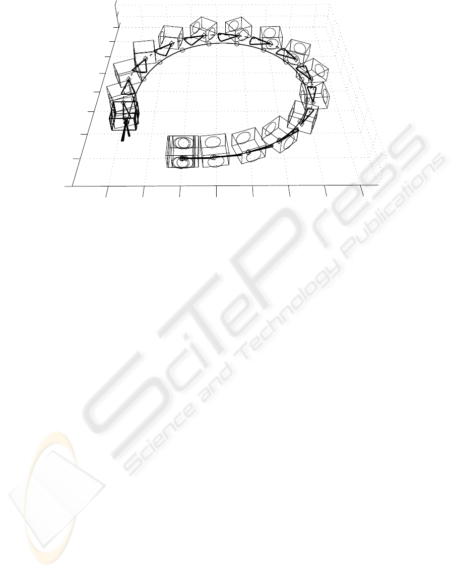
To show the performance of the algorithm at larger
centripetal accelerations and larger side-slip angles,
a sharp turn with a minimum radius of 0.29m at a
velocity of 1.1ms
−2
is performed, leading to a peak
side-slip angle of 45
◦
, Fig. 10.
A certain position error has to be accepted, but
as soon as the side-acceleration (and with it the
side-slip) diminishes, the error is compensated.
ICINCO 2005 - ROBOTICS AND AUTOMATION
118

−0.2
−0.1
0
0.1
0.2
0.3
0.4
0.5
−0.1
0
0.1
0.2
0.3
0.4
0.5
0.6
0.7
0
0.05
0.1
x
y
Figure 10: 3D-visualization of the robot sliding through a sharp turn
In a first practical test, the algorithm, written in
C, was executed on a 600MHz-clock-rate Blackfin
BF533 DSP. The calculation time consumed during
each sampling interval is well below the duration of
the interval.
7 CONCLUSION
A robust and universally applicable tracking control
algorithm is presented, that suffers under none of the
drawbacks inherent to the various approaches found
in literature.
The presented tracking algorithm performs very
well even under severe disturbances in a simulation.
The state feedback controller with integration of
the control error of the inner loop makes the system
very robust against modeling inaccuracies.
The optimization in the outer loop does not con-
tain any model assumptions except for the kinematic
equations, which are not subject to any uncertainties,
and is therefore (depending on the tuning parameters)
very robust against changing ground conditions.
Although the algorithm was developed for the class
of unicycle-type mobile robots or 2WDD(two-wheel-
differential-drive)-robots, it can easily be adapted to
be used for four-wheelers with one steered axle. Only
the velocity dynamics would have to be modified.
REFERENCES
Bloch, A. and Drakunov, S. (1994). Stabilization of a Non-
holonomic System via Sliding Modes. IEEE Confer-
ence on Decision and Control.
Brockett, R. W. (1983). Differential Geometric Control
Theory, chapter Asymptotic Stability and Feedback
Stabilization. Birkhauser.
Hespanha, J. P. and Morse, A. S. (1996). Stabilization of
Nonholonomic Integrators via Logic-Based Switch-
ing. Automatica’s Special Issue on Hybrid Systems,
to appear.
Isermann, R. (1987). Digitale Regelsysteme, volume 1.
Springer.
Isidori, A. (1989). Nonlinear Control Systems. Springer.
Mayne, D. Q., Rawlings, J. B., Rao, C. V., and Scokaert,
P. O. M. (2000). Constrained Model Predictive Con-
trol: Stability and Optimality. Automatica, (36):789–
814.
Norgaard, M., Ravn, O., and Poulsen, N. K. (1999). Neural
Networks for Modelling and Control of Dynamic Sys-
tems. Springer.
Oriolo, G., De Luca, A., and Vendittelli, M. (2002). WMR
Control Via Dynamic Feedback Linearization: De-
sign, Implementation, and Experimental Validation.
IEEE Transactions on Control Systems Technology,
10(6):835–851.
Samson, C. (1995). Control of Chained Systems. Appli-
cation to Path Following and Time-Varying Point-
Stabilization of Mobile Robots. IEEE Transactions
on Automatic Control, 40(1):64–77.
Seyr, M. and Jakubek, S. (2005). Neural Network Predictive
Trajectory Tracking of an Autonomous Two-Wheeled
Mobile Robot. In IFAC05 conference proceedings.
MOBILE ROBOT PREDICTIVE TRAJECTORY TRACKING
119