
ROBUST STABILITY ANALYSIS OF SINGULARLY
PERTURBED MAGNETIC SUSPENSION SYSTEMS
§
Nan-Chyuan Tsai, Chien-Ting Chen
Department of Mechanical Engineering, National Cheng Kung University,
Tainan City, 701,Taiwan
Keywords: Singular perturbation, Two-time-scale systems, Kharitonov Theorem.
Abstract: For a singularly perturbed magnetic suspension system, two kinds of state feedback controllers are
synthesized to account for the inherent instability of the open-loop plant with two-time-scale properties.
Kharitonov polynomials, extremal vertex and uncertain Nyquist plot are employed to examine the maximum
tolerance against system parameters uncertainties such that the stability of the closed-loop system is still
retained. Experimental simulations are reported to illustrate the robustness of designed controllers both in
stability and performance. At last, Interlacing Theorem is introduced to analyze the stability of uncertain
suspension systems via the characteristic interval polynomials. It is found that identical results are obtained,
in comparison with extremal vertex approach.
1 INTRODUCTION
In general, two-time-scale systems are not
uncommon in practice, such as electro-mechanical
systems, power engineering and so on. The major
feature of this kind of singularly perturbed systems
is the eigenvalues of the plant are located distinctly
apart into two sectors: one near the origin on
complex frequency plane and the other far away. In
other words, two-time-scale system can be analyzed
as a coupled system composed by a slow subsystem
and a fast subsystem.
The singular perturbation technique is employed
to decouple the slow subsystem and the fast
subsystem by choosing an appropriate coordinate
transformation such that the controller for the two-
time-scale system can be designed individually by
two uncoupled models at first and then composed
together. Numerous researchers had applied this
concept to synthesize the singularly perturbed
industrial control systems. Vournas et al. reported
to design the generator voltage regulator by singular
perturbation method (Vournas, 1995). Flexible
robot links have been discussed and presented
frequently by this technique (Spong, 1989).
Suspension of quarter-car model has been analyzed
by two-time-scale model (Salman, 1988). However,
the robustness in singularly perturbed suspension
has not much been addressed.
In this work, the magnetic suspension system is
investigated both in robust stability analysis and in
control synthesis. The parasitic parameter, that is
crucial in singular perturbation system, is found to
be strongly related to the inductance value of the
electromagnet. Unfortunately, some of the
parameters are not only of small values, but also
inherent in uncertainties. Therefore, Kharitonov
Theorem is introduced to analyze how robust the
closed-loop system will be, from the viewpoint of
stability with respect to system parameters
variations. Two kinds of controllers are synthesized
and compared in experimental simulations. It is
concluded that the designed controllers exhibit
dramatically robust enough to account for parameter
uncertainties up to
± 50% variation away from the
nominal values, while the performances of the
closed-loop system are not detrimentally degraded.
2 PROBLEM FORMULATION
The magnetic suspension system (Fujita, 1995),
shown in Figure 1, is inherently unstable so that a
closed-loop control strategy is required.
166
Tsai N. and Chen C. (2005).
ROBUST STABILITY ANALYSIS OF SINGULARLY PERTURBED MAGNETIC SUSPENSION SYSTEMS.
In Proceedings of the Second International Conference on Informatics in Control, Automation and Robotics - Signal Processing, Systems Modeling and
Control, pages 166-172
DOI: 10.5220/0001188001660172
Copyright
c
SciTePress
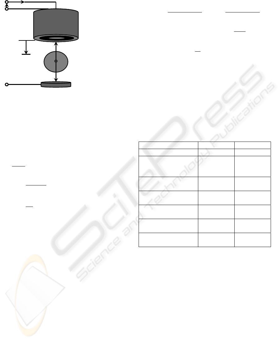
Table 1: Parameters
2.1 Equation of Motion
The single degree-of-freedom dynamic model of
magnetic suspension can be easily described as
follows:
fmg
dt
pd
m −=
2
2
(1)
2
0
)(
pp
i
kf
+
= (2)
e
dt
di
LRi =+
(3)
where f is the magnetic control force that is
proportional to the square of coil current, i(t), and
inversely proportional to the square of total air gap,
p(t)+ p
0
. k is a constant. p
0
is denoted as the offset
determined by the measurement instruments and
sensor locations.
e
represents the exerted control
voltage applied via amplifiers set on the coil of
electromagnets. The interested parameters are
tentatively considered as constants and listed in
Table 1. The linearized state space model can be
obtained by taking Taylor’s Expansion around (
P+p
0
, I ). I is the steady-state control current as the
air gap reaches ( P + p
0
) that is the quasi-steady-
state value at which the gravity of the control force
is balanced.
uBXAX +=
(4)
XCy = (5)
⎥
⎥
⎥
⎥
⎥
⎥
⎦
⎤
⎢
⎢
⎢
⎢
⎢
⎢
⎣
⎡
−
+
−
+
=
L
R
pPm
kI
pPm
kI
A
00
)(
2
0
)(
2
010
2
0
3
0
2
(6)
⎥
⎦
⎤
⎢
⎣
⎡
=
L
T
B
1
00
(7)
[]
001=C (8)
[
]
ippX
T
ˆ
ˆˆ
=
(9a)
)()(
ˆ
0
pPtpp +−= (9b)
Itii −= )(
ˆ
(9c)
The measurement is the incremental
displacement,
p
ˆ
, only, experimentally available
from an eddy-current gap sensor.
Parameter Symbol Value
Mass of the iron ball m [kg] 1.75
Steady-state gap
between the magnet
and the iron ball
P [m] 2×10
-2
Steady-state current of
the electromagnet
I [A] 1.06
Inductance of the
electromagnet
L [H]
5.08×10
-2
Resistance of the
electromagnet
R [Ω] 23.2
Constants determined
by experiment
p
0
[m] 10-4
Coefficient of the
electromagnetic force
k [Nm
2
/A
2
] 2.9×10
-4
2.2 Singular Perturbation System
From Eq.(4) and the actual experimental data in
Table 1, it is obvious to find that the poles, {
± 7.5355, -456.6929}, of the studied open-loop
magnetic suspension system are located into two
groups that are far away from each other. That is,
the pole, “-456.6929”, is about 65 times in distance
from the origin of complex frequency plane,
compared with the poles, {7.5355, -7.5355}. It
implies that in time domain the plant has the two-
time-scale property with respect to the state
variables. Hence, Eq.(4)-(9) can be rewritten as the
standard form of singular perturbation model as
follows (Kokotovic, 1986):
uBzAxAx
11211
++=
(10)
f
mg
Electromagnet
Iron Ball
Gap Sensor
i
e
p
f
mg
Electromagnet
Iron Ball
Gap Sensor
i
e
p
Figure 1: Magnetic suspension system.
ROBUST STABILITY ANALYSIS OF SINGULARLY PERTURBED MAGNETIC SUSPENSION SYSTEMS
167
uBzAxAz
22221
++=
ε
(11)
zCxCy
21
+= (12)
⎥
⎥
⎦
⎤
⎢
⎢
⎣
⎡
+
=
0
)(
2
10
3
0
2
11
pPm
kI
A
(13a)
⎥
⎦
⎤
⎢
⎣
⎡
+
−=
2
0
12
)(
2
0
pPm
kI
A
T
(13b)
]00[
21
=A (13c)
[]
RA −=
22
(13d)
[]
00
1
=
T
B (13e)
1
2
=
T
B (13f)
]01[
1
=C (13g)
0
2
=C (13h)
L=
ε
(13i)
]
ˆˆ
[ ppx
T
= (13j)
iz
ˆ
= (13k)
where
ε
is called as the perturbation parameter that
is assumed as a positive scalar but, to some extent,
close to zero. The reduced model can be constructed
by letting
0=
ε
.
)()()( tuBtxAtx
sssss
+=
(14a)
)()()( tuDtxCty
sssss
+= (14b)
)(
221
1
22 sss
uBxAAz +−=
−
(14c)
where
21
1
221211
AAAAA
s
−
−= (15a)
2
1
22121
BAABB
s
−
−= (15b)
21
1
2221
AACCC
s
−
−= (15c)
2
1
222
BACD
s
−
−= (15d)
x
s
and z
s
are the state variables of reduced model. y
s
is the output of the slow subsystem. The overall
controller can be designed individually on the bases
of slow subsystem model and fast subsystem. For
example, if the state feedback control strategy is
taken, then:
(a) on the base of slow subsystem,
ss
xHu
0
= (16)
That is, to design
s
u is based on Eq.(14a) and
Eq.(14b) only.
(b) on the base of fast subsystem,
ff
zHu
2
= (17)
That is, to design
f
u is based on Eq.(14c) and the
fast subsystem defined as follows:
fff
uBzAz
222
+=
ε
(18a)
ff
zCy
2
= (18b)
where
sf
zzz −= ,
sf
uuu −= .
To sum up, the overall state feedback can be
constructed by direct composition by addition.
)]([
0221
1
222
0
20
xHBxAAzH
xH
zHxH
uuu
fs
fS
+++
=
+=
+=
−
zHxH
21
+= (19)
where
))(
21
1
22202
1
2221
AAHHBAHIH
−−
++=
Its schematic control loops are shown in Figure 2.
3 CONTROLLER DESIGN ON
SINGULARLY PERTURBED
SUSPENSTION SYSTEMS
It has been well known that an appropriate controller
design on the reduced perturbation model can be
applied on the actual suspension systems. The
errors, of states or system output, are restricted in
first-order zero approximation, i.e.,
)(
ε
O , due to
effect caused by reduction from exact model as long
as the fast subsystem matrix of perturbed state-space
model, A
22
(x, z, t) , is Hurwitz (Saksena, 1984). In
other words, partial state feedback can be utilized to
ensure the asymptotic stability and performance of
the actual system. If the state feedback law is
described as follows:
[]
[]
TTT
zxHHu
21
= (20)
Two kinds of feedback controllers are designed
and compared in this work: Eigenvalues Assignment
and Near-optimal approach.
Figure 2
:
Composite state feedback
.
uB
z
x
A
z
x
+
⎥
⎦
⎤
⎢
⎣
⎡
=
⎥
⎦
⎤
⎢
⎣
⎡
ε
+
+
x
z
2
H
1
H
u
uB
z
x
A
z
x
+
⎥
⎦
⎤
⎢
⎣
⎡
=
⎥
⎦
⎤
⎢
⎣
⎡
ε
+
+
x
z
2
H
1
H
u
ICINCO 2005 - SIGNAL PROCESSING, SYSTEMS MODELING AND CONTROL
168
3.1 Eigenvalue Assignment
Under assumption of controllability of reduced slow
subsystem, the eigenvalues can be assigned
anywhere on the complex frequency plane. At least
the unstable poles can be moved to the stable region
if the slow subsystem is stabilizable. The feedback
gain matrix is denoted as H that will be used later.
3.2 Near-Optimal Approach
A near-optimal linear quadratic regulator is designed
against the performance index:
dtuRuyyJ
s
T
ss
T
ss
)(
2
1
0
∫
∞
+= (21)
where the subscript”s” represents the approach is
undertaken in slow-state model. The associated
steady-state matrix Riccati Equation can be obtained
by traditional optimization methodology.
s
T
ss
T
s
s
T
sss
s
T
s
T
sss
s
T
ssss
CDRDIC
PBRBP
PCDRBA
CDRBAP
)(
)(
)(0
1
0
1
0
1
0
1
0
−
−
−
−
−−
+
−−
−−=
(22)
where
s
T
s
DDRR +=
0
(23)
Therefore, the control command is generated by the
feedback law:
ss
T
ss
T
ss
xPBCDRu )(
1
0
+−=
−
(24)
4 SIMULATION RESULTS
As a gap sensor, a standard induction probe of eddy-
current type is placed closely near the bottom of the
iron ball in Figure 1. An electromagnet, of ”EI”
shape in geometry, is used to generate magnetic
force near the top of the controlled mass. A digital
signal processor DSP-based real-time controller is
implemented with TMS320C240. The data
acquisition board MSP-77230 consists of a set of 12-
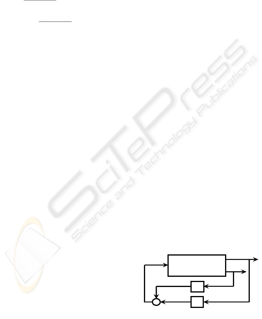
bit A/D and D/A converters. With non-zero initial
conditions, i.e., the state has an initial deviation, the
closed-loop suspension system is regulated to be
zero within 0.5 second either by near-optimal
controller or eigenvalue assignment design, shown
in Figure 3a. The associated required control is
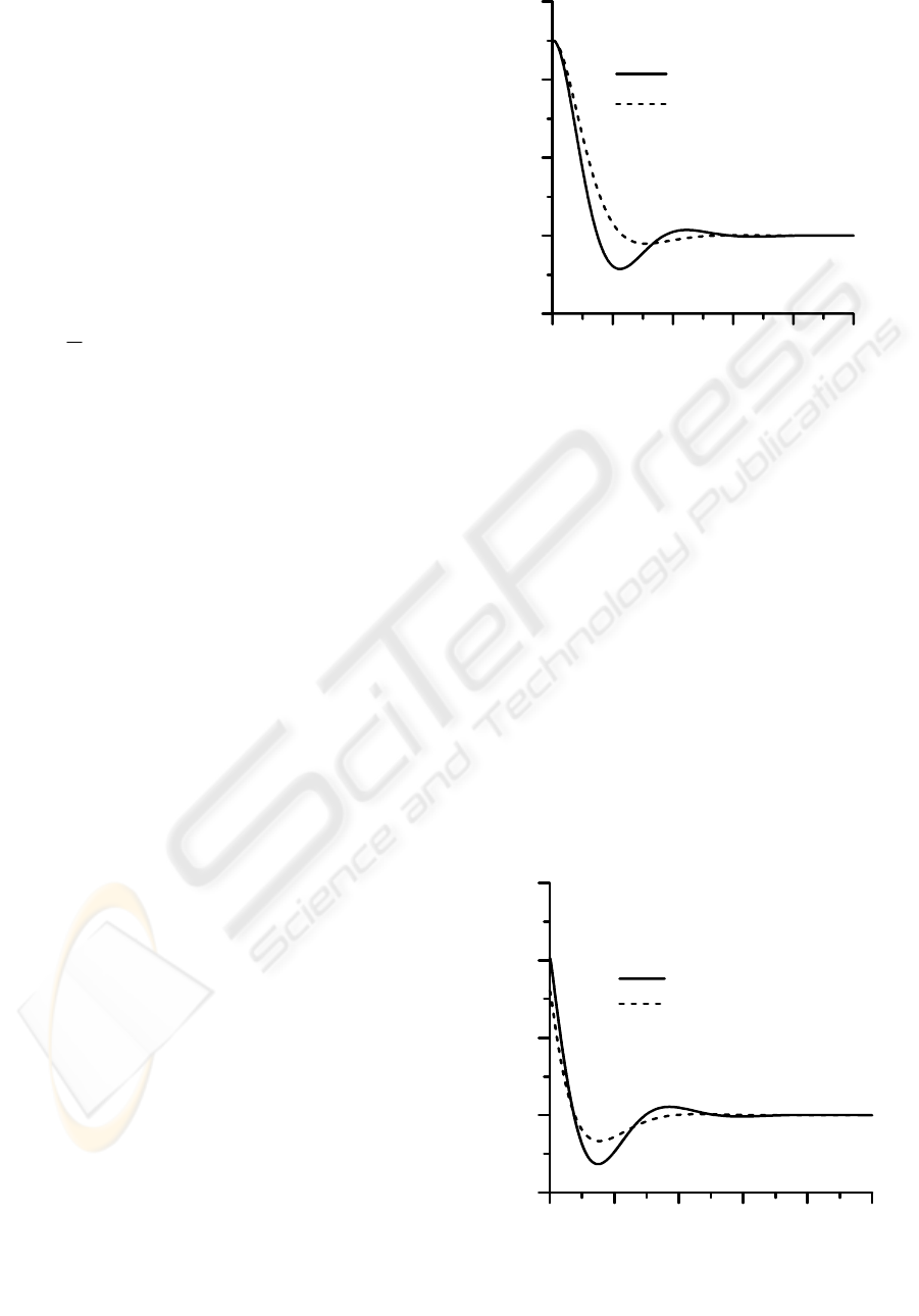
plotted in Figure 3b. From the viewpoint if stiffness
of closed-loop system, a unit step response is
examined and shown in Figure 4. quick response.
Though the performance of the closed-loop system
is degraded, subjected to
± 50% parameter variation
in inductance L, under the identical LQ Controller
designed on the base of nominal value, it is not
detrimental and exhibits strongly robust, shown in
Figure 5.
5 ROBUST STABILITY
ANALYSIS
The main reasons that cause singular perturbation
are: (i) presence of relatively small parasitic
parameters, and (ii) inclusion of hign gain control
loops. In this study on magnetic suspension
systems, it is evident that the inductance value of the
electro-magnet is relatively small so that the singular
perturbation problem emerges. Even worse is that
the inductance value changes in time. Practically, the
Figure 3a: Time response under non-zero initial
condition
0.00 0.20 0.40 0.60 0.80 1.00
Time (sec)
-0.00
0.00
0.00
0.00
0.00
State x
1
(meter)
Eigenvalue Assignment
Near-optimal Control
0.00 0.20 0.40 0.60 0.80 1.00
Time (sec)
-2.00
0.00
2.00
4.00
6.00
Control Current (A)
Eigenvalue Assignment
Near Optimal Control
Figure 3b: Control current for linear quadratic
regulation
ROBUST STABILITY ANALYSIS OF SINGULARLY PERTURBED MAGNETIC SUSPENSION SYSTEMS
169
variation of the inductance can be constrained by a
preset pair of upper and lower limits. The
parameters uncertainties and resulted robust stability
problems are hereby to be investigated as follows.
Applying the concepts of polynomial vertex and
Kharitonov segments (Bhattacharyya, 1995), totally
four Kharitonov Polynomials are to be
simultaneously examined to determine the closed-
loop stability region against inductance uncertainty.
The Eigenvalue Assignment approach is taken as an
illustrative example in this report to analyze the
stability robustness of the closed-loop system.
The closed-loop system matrix under state
feedback can be expressed in the form:
)(
ˆ
HBAA −= (25)
Since the open-loop is a third-order system, the
characteristic polynomial of the closed-loop system
can be described as follows:
3
3
2
210
)( ssss
δδδδδ
+++= (26)
If each of the parameters of the characteristic
polynomial varies between two limits, i.e.,
[]
000
,
βαδ
∈ ,
[]
111
,
βαδ
∈ ,
[]
222
,
βαδ
∈ ,
[]
333
,
βαδ
∈ , then the four Kharitonov
Polynomial can be obtained:
3
3
2
210
1
)( ssssK
βββα
+++= (27a)
3
3
2
210
2
)( ssssK
αββα
+++= (27b)
3
3
2
210
3
)( ssssK
βααβ
+++= (27c)
3
3
2
210
4
)( ssssK
ααββ
+++= (27d)
These four extremal polynomials are the complete
independent characteristic polynomials to be
examined for ensurance of stability of closed-loop
uncertain systems. The other twelve extremal
polynomials are proved redundant and can be
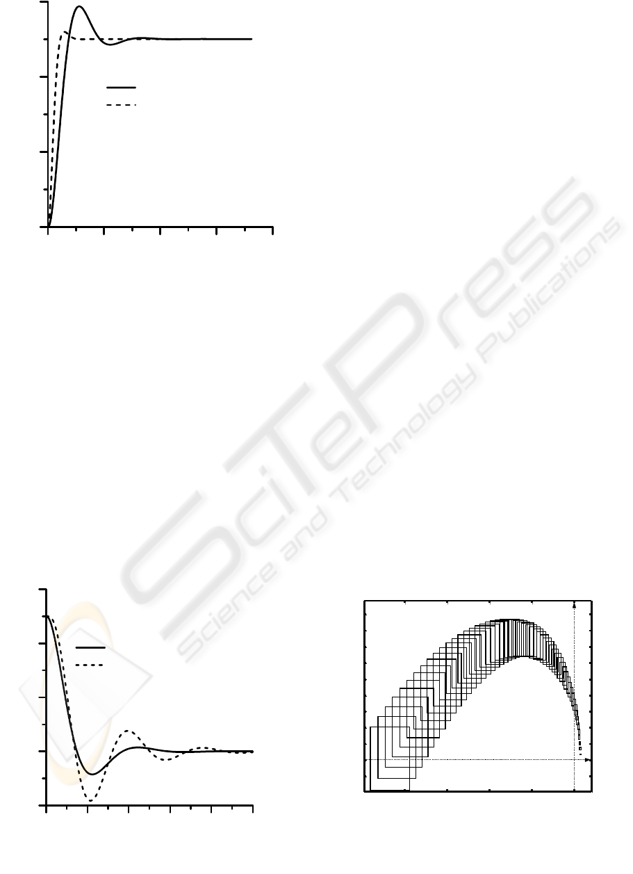
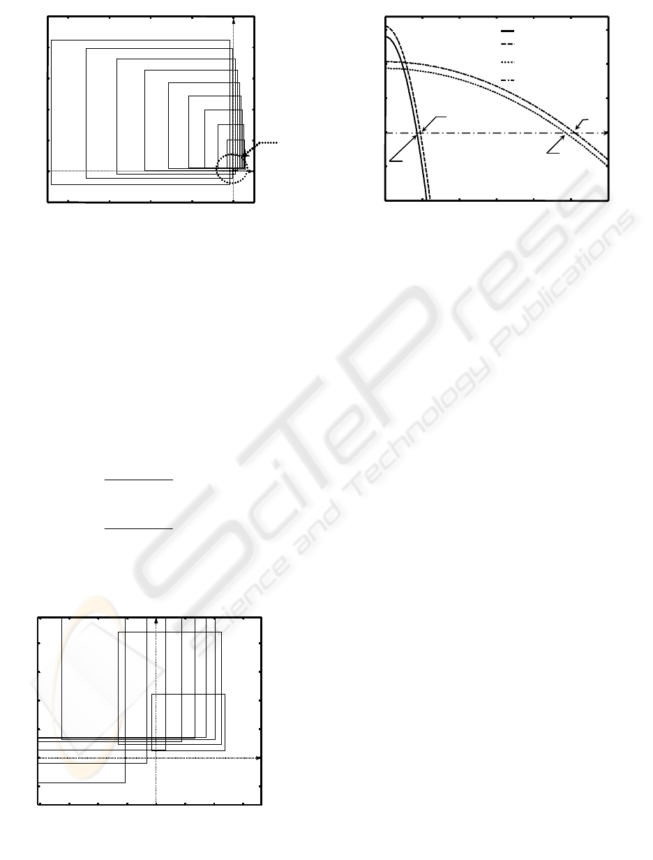
dumped at all (Bhattacharyya, 1995).The effect of
parameter uncertainties in Nyquist plot of closed-
loop system are shown in Figure 6 and Figure 7,
with
± 5% and ± 50% variation each, with respect
to the nominal parameter value, respectively. These
two figures conclude that the controller, designed by
Eigenvalue Assignment, is robust in stability, with
maximum tolerance of
±
50% parameter variations.
In other words, when the parameter uncertainty
exceeds beyond
±
50%, the closed-loop control
system becomes unstable.
Another approach is to apply Interlacing Theorem
(Bhattacharyya, 1995). The odd-order and even-
order extremal polynomials of the closed-loop
systems are defined as follows:
0.00 0.40 0.80 1.20 1.60
Time (sec)
0.00
0.40
0.80
1.20
State x
1
(meter)
Eigenvalue Assignment
Near Optimal Control
Figure 4
:
Step response
-0.00
0.00
0.00
0.00
0.00
State x
1
(meter)
0.00 0.20 0.40 0.60 0.80 1.00
Time (sec)
nominal value ( of inductance L )
+ 50% parameter variation ( of inductance L )
Figure 5
:
R
obust performance of regulation
-4 -3 -2 -1 0
x 10
6
-0.5
0
0.5
1
1.5
2
2.5
3
3.5
4
4.5
x 10
5
Real
Imag.
Image Sets of Kharitonov Boxes
Figure 6
:
Nyquist plot for uncertainties up to
±
5
%.
ICINCO 2005 - SIGNAL PROCESSING, SYSTEMS MODELING AND CONTROL
170
2
20max
)( ssK
even
αβ
+= (28a)
2
20min
)( ssK
even
βα
+= (28b)
3
31max
)( sssK
odd
αβ
+= (28c)
3
31min
)( sssK
odd
βα
+= (28d)
Let
w
j
s
= , the Equation set (28) can be rewritten
in real or imaginary part as follows:
2
20maxmax
)()( wwjKwK
eveneven
αβ
−== (29a)
2
20minmin
)()( wwjKwK
eveneven
βα
−== (29b)
2
31
max
max
)(
)( w
wj
wjK
wK
odd
odd
αβ
+== (29c)
2
31
min
min
)(
)( w
wj
wjK
wK
odd
odd
βα
+== (29d)
The values of the above four extremal
polynomials versus frequency are shown in Figure 8.
The intersections of extremal
polynomials,
)(
max
wK
even
, )(
min
wK
even
, )(
max
wK
odd
and
)(
min
wK
odd
, and frequency axis are Q
1
, Q
2
, Q
3
and Q
4
respectively. According to Interlacing Theorem, the
inequality 0<Q
1
<Q
2
<Q
3
<Q
4
implies that the closed-
loop system retains stable under the parameter
uncertainties
± 5% each. This result is identical to
the one from uncertain Nyquist plot.
6 CONCLUSION
The inductance value in magnetic suspension system
plays a crucial role for singular perturbation analysis
and synthesis. Since the two-time-scale properties
dominate the extent of singularly perturbed stability
and performance, the robustness with respect to the
perturbation parameter has to be examined. The
Kharitonov Polynomials and Interlacing Theorem
both verifies that the controller design, either by
eigenvalue assignment or near-optimal approach,
would retain robust in stability. It has been also
proved by experimental simulations. The
performance, of the closed-loop system in the worst
case of
± 50% inductance variation, is not greatly
deteriorated. This implies that the performance
robustness is also achieved.
-8 -6 -4 -2 0
x 10
6
-0.5
0
0.5
1
1.5
2
2.5
x 10
6
Real
Imag.
Image Sets of Kharitonov Boxes
Detail A
-8 -6 -4 -2 0
x 10
6
-0.5
0
0.5
1
1.5
2
2.5
x 10
6
Real
Imag.
Image Sets of Kharitonov Boxes
Detail A
Detail “A”
-8 -6 -4 -2 0
x 10
6
-0.5
0
0.5
1
1.5
2
2.5
x 10
6
Real
Imag.
Image Sets of Kharitonov Boxes
-8 -6 -4 -2 0
x 10
6
-0.5
0
0.5
1
1.5
2
2.5
x 10
6
Real
Imag.
Image Sets of Kharitonov Boxes
Detail ADetail A
-8 -6 -4 -2 0
x 10
6
-0.5
0
0.5
1
1.5
2
2.5
x 10
6
Real
Imag.
Image Sets of Kharitonov Boxes
-8 -6 -4 -2 0
x 10
6
-0.5
0
0.5
1
1.5
2
2.5
x 10
6
Real
Imag.
Image Sets of Kharitonov Boxes
Detail A
Detail “A”
Figure
7a
:
Nyquist plot f
or uncertainties up to
±
5
0
%.
Figure 7b
:
Detail of
”
A
”
.
-8 -6 -4 -2 0 2 4 6
x 10
5
-1
0
1
2
3
4
x 10
5
Real
Imag.
Image Sets of Kharitonov Boxes
0 20 40 60 80 100 120
-1
-0.5
0
0.5
1
1.5
x 10
5
w (rad/sec)
Q
2
Q
1
Q
4
Q
3
K
e
min
(w)
K
e
max
(w)
10 K
o
min
(w)
×
10 K
o
max
(w)
×
Real
0 20 40 60 80 100 120
-1
-0.5
0
0.5
1
1.5
x 10
5
w (rad/sec)
Q
2
Q
1
Q
4
Q
3
K
e
min
(w)
K
e
max
(w)
10 K
o
min
(w)
×
10 K
o
min
(w)
×
10 K
o
max
(w)
×
Real
Figure 8
:
Interlacing of extremal polynomials.
ROBUST STABILITY ANALYSIS OF SINGULARLY PERTURBED MAGNETIC SUSPENSION SYSTEMS
171

REFERENCES
Bhattacharyya, S. P., Chapellat, H., Keel, L. H.
1995.Robust Control: The Parametric Approach,
Prentice Hall PTR.
Chow, J. H., Kokotovic, P. V. 1976. A Decomposition of
Near-Optimal Regulators for Systems with Slow and
Fast Modes. In IEEE Trans. Automat.Contr. vol. AC-
21, pp. 701-705.
Fujita, M., Namerikawa, T., Matsumura, F., Uchida, K.
1995.µ-Synthesis of an Electromgnetic Suspension
System. In IEEE Trans. Automat Contr. vol. 40, pp.
530-536.
Khorrami, F., Ozguner, U. 1988. Perturbation method in
control of flexible link manipulators. IEEE. pp.310-
315
Kokotovic, P. V., Khalil, H. K., O’Reilly, J. O. 1986.
Singular Perturbation Methods in Control : Analysis
and Design, Academic Press. New York.
Lewis, F. L., Vandegrift, M., 1993. Flexible robot arm
control by a feedback linearization/singular
perturbation approach. In IEEE International
Conference on Robotics and Automation. vol. 3,
pp.729-736.
Salman, M. A., Lee, A. Y., Boustany, N. M. 1988.
Reduced order design of active suspension control. In
Proceedings of the IEEE Conference on Decision and
Control Including The Symposium on Adaptive
Processes. pp.1038-1043.
Saksena, V. R., O’Reilly, J. O., Kokotovic, P. V. 1984.
Singular perturbations and time-scale methods in the
control theory. In Automatic. vol. 20, pp.273-293.
Spong, M. W, 1989. On the force control problem for
flexible joint manipulators. In IEEE Transactions on
Automatic Control. vol. 34, pp.107-111.
Vournas, C. D., Sauer, P. W., and Pai, M. A, 1995. Time-
scale decomposition in voltage stability analysis of
power systems. In IEEE Conference on Decision and
Control, vol. 4, pp.3459-3464.
ICINCO 2005 - SIGNAL PROCESSING, SYSTEMS MODELING AND CONTROL
172
