KINEMATIC MODELING OF STEWART-GOUGH PLATFORMS
Pedro Cruz, Ricardo Ferreira
Institute for Systems and Robotics
Av. Rovisco Pais 1, 1049-001 Lisboa, Portugal
Jo
˜
ao Silva Sequeira
Instituto Superior T
´
ecnico
Institute for Systems and Robotics
Av. Rovisco Pais 1, 1049-001 Lisboa, Portugal
Keywords:
Parallel robots, Direct kinematics, Inverse kinematics.
Abstract:
This paper describes a method to solve the direct kinematics of a generic Stewart-Gough manipulators. The
method is formulated in terms of a search in the space of rigid body transformations. The underlying idea is
that the solutions of the direct kinematics can be obtained by moving the end-effector body according rotations
and translations and accounting for the rigidity conditions.
The paper presents simulation results for a 6-3 Stewart-Gough robot.
1 INTRODUCTION
This paper presents a method to solve the direct kine-
matics of Stewart-Gough robots. This work aims at
assessing the use of numerical algorithms for a real
time application to the control of such robots.
The use of parallel robots undergoes a renewed in-
terest nowadays due to the variety of possible practi-
cal applications. Parallel robot structures can be de-
signed which are specially tailored to handle heavy
loads with accurate positioning. Roughly, position-
ing errors in serial kinematic chains tends to propa-
gate additively throughout the chain links. This is not
the case with parallel manipulators, which are con-
sequently capable of performing positioning tasks to
a high degree of accuracy. Furthermore, the paral-
lel structure inherently distributes the forces/torques
by the actuators giving this class of robots high band-
width dynamic characteristics. Typical applications
include flight simulators, shaking tables (used in sim-
ulation of the effects of earthquakes in building struc-
tures), support structures for the accuracy position-
ing of instrumentation, medical instrumentation and
even entertainment devices (see for instance (Merlet,
2000)).
The generic Stewart-Gough platform is composed
of two rigid bodies connected through a number of
prismatic actuators as in a parallel arrangement of
kinematic chains. Usually six actuators are used,
pairing arbitrary points in the two bodies. The
linkages between the actuators and the bodies are
made through non-actuated universal or ball-in-socket
joints.
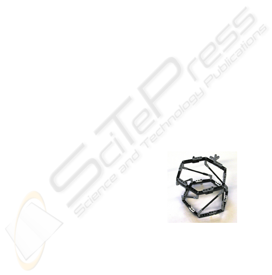
Figure 1 presents a Lego-based physical model of a
Stewart-Gough platform with six connecting rods of
fixed length in place of the linear actuators.
Figure 1: A Stewart-Gough platform model constructed us-
ing Lego
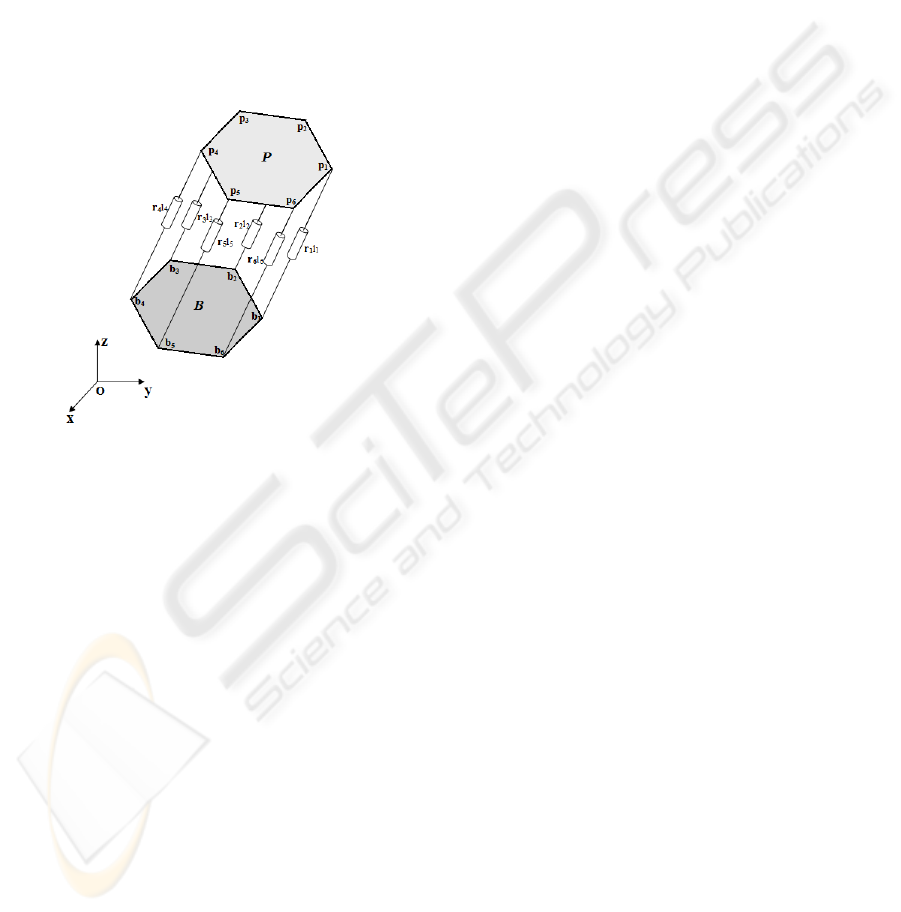
Figure 2 illustrates the terminology used in the paper.
The two bodies are denoted by B and P and the linear
actuators connect them at the anchor points denoted
by {b
1
,...,b
6
} and {p
1
,...,p
6
}, respectively in B
and P . For the sake of simplicity, the polygonal line
joining the b
i
points and the polygonal line joining
the p
i
points, are assumed to form simple polygons.
In the sequel B is assumed to be rigidly connected
93
Cruz P., Ferreira R. and Silva Sequeira J. (2005).
KINEMATIC MODELING OF STEWART-GOUGH PLATFORMS.
In Proceedings of the Second International Conference on Informatics in Control, Automation and Robotics - Robotics and Automation, pages 93-99
DOI: 10.5220/0001189900930099
Copyright
c
 SciTePress

to the ground, as the base of the robot. The body
P moves according to the joint values and the kine-
matic constraints. The actuator lengths are denoted
by l
i
,i=1,...,6. The i-th actuator connects the
points b
i
and p
i
and has length l
i
.
Unlike serial manipulators, the direct kinematics of
generic parallel manipulators can not be easily writ-
ten in closed form. Numerical methods are often used
to determine the position and attitude of the P body
from the set of joint variables (the lengths of the actu-
ators).
Figure 2: A generic Stewart-Gough platform
The direct kinematics of a generic Stewart-Gough
platform has often multiple solutions. For instance,
the general Stewart-Gough platform can have 40 real
solutions, (Dietmaier, 1998). Practical applications of
direct kinematics, e.g, in robot control architectures,
often require a one to one correspondence between
subsets in the spaces of joint variables and positions
and attitudes. Therefore, a relevant aspect in the study
of the kinematics of parallel robots is related with the
ability of the kinematics solution methods to converge
to a particular solution.
Various approaches to the computation of the kine-
matics of Stewart-Gough robots have been presented
in the literature. In (Jakobovi
´
c and Budin, 2002) the
direct kinematics problem is addressed by solving six
optimization problems, one for each actuator. Algo-
rithms like Powell’s method, Hooke-Jeeves’, steep-
est descent with constant update steps and Fletcher-
Powell’s were used to solve those problems. The di-
rect kinematics is also addressed as an optimization
problem in (Hopkins, 2002), solved using a Newton-
Raphson method. The work in (Hopkins, 2002) is
integrated in a control architecture. A hybrid strat-
egy using neural networks and Newton-Raphson tech-
niques is proposed in (Parikh and Lam, 2005). In this
strategy the neural network stage is used to obtain the
initial estimate for the Newton-Raphson method. Dy-
namic modeling, a fundamental aspect for high per-
formance control, has been addressed in (Khalil and
S., 2004).
This paper presents an algorithm that describes the
motion of the P body as a rigid body transforma-
tion, i.e., through rotations and translations. Newton’s
method is used to compute the rigid body transforma-
tion matrix that corresponds to the desired solution
of the direct kinematics of Stewart-Gough platforms.
Simulation results are obtained from one special class
of Stewart-Gough platform 6-3/\
3
configuration (the
notation in (Merlet, 2000) is followed hereafter to de-
scribe the organisation of the actuators in the robot).
The direct kinematics problem is formalized as an
optimization problem and simulation results obtained
are presented.
The paper is organized as follows. Section 2 de-
scribes the direct kinematics problem (the inverse
kinematics is trivial) in the space of rigid body trans-
formations. Section 3 describes a set of simulation
experiments. Section 4 presents the conclusions of
the paper and ongoing work.
2 KINEMATICS MODELING
Table 1 details the notation used in the paper to for-
mulate the kinematics of the robot.
Table 1: Notation used in the paper
l
i
a scalar standing for the i-th
actuator length
p
i
=(p
x
i
,p
y
i
,p
z
i
) point in R
3
belonging to P
b
i
=(b
x
i
,b
y
i
,b
z
i
) point in R
3
belonging B
r
i
unit vector in R
3
¯p
i
the “usual” inclusion of p
i
in the projective space P
3
q
i
representation of point p
i
described in a local refer-
ence frame (see Figure 3)
Figure 3 illustrates relations between the coordi-
nate reference frames assigned to the rigid bodies that
form the robot.
Assuming the rigidity of the two bodies B and P ,
the kinematics of the robot is completely described by
the set of equations,
ICINCO 2005 - ROBOTICS AND AUTOMATION
94

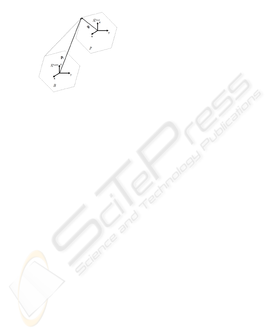
Figure 3: Relations between reference frames
(p
x
i
− b
x
i
)
2
+(p
y
i
− b
y
i
)
2
+(p
z
i
− b
z
i
)
2
= l
2
i
,
i =1,...,6 (1)
meaning that, for any actuator, any achievable config-
uration must lie in a 2D ball embedded in R
3
.
Expanding the square terms in the lefthand side of
(1) the expression can be written as
¯p
T
i
C
i
(b
i
,l
i
) ¯p
i
=0,i=1,...,6 (2)
where C
i
is a matrix relating the i-th actuator and the
B body defined as
C
i
=
⎡
⎢
⎣
100 −b
x
i
010 −b
y
i
001 −b
z
i
−b
x
i
−b
y
i
−b
z
i
b
T
i
b
i
− l
2
i
⎤
⎥
⎦
(3)
The solution of the direct kinematics problem ex-
pressed by (2) can be obtained by moving the P body
in the 3D space. This amounts to finding the adequate
rotation and translation such that (2) has a solution.
Alternatively, this can also be seen as finding a new
reference frame where to describe the p
i
solutions of
(2), that is,
¯p
i
= T¯q
i
(4)
where ¯q
i
describes ¯p
i
in a local reference frame and
T ∈ SE(3) is the homogeneous transformation ma-
trix given by
T =

Rt
0 1

(5)
with R standing for a rotation matrix and t standing
for the displacement between the origins of the two
reference frames. Equation (2) can then be written as
¯q
T
i
T
T
C
i
(b
i
,l
i
) T¯q
i
=0
i =1,...,6 (6)
In addition, it is also necessary to ensure that the
structure of of the elements in T is preserved, namely
that R ∈ SO(3). Given the homogeneous structure of
(6) this condition can be relaxed to R ∈ O(3) yield-
ing the following 9 additional constraints,
R
T
R = I
3
⇐⇒ [
I0
] T
T

I
0

[
I0
] T

I
0

= I
3
⇐⇒ I
3×4
T
T
DTI
4×3
= I
3
All the 15 restrictions have the general form
g
i
(T)=a
i
T
T
T
C
i
Tb
i
− d
i
=0 (7)
and hence the solution of the forward kinematics
amounts to find a solution for a non-linear system of
15 equations and 12 unknowns.
Expression (7) is thus the formulation of the di-
rect kinematics problem in the space of homogeneous
transformations.
2.1 Solution by Newton’s method
To obtain a solution of (7) the g
i
(T) is expanded in
Taylor series, retaining only the first order terms,
g
i
(T + H)=g
i
(T)+
(∇g
i
)
T


T
vec (H)+O( vec(H)
2
) (8)
where ∇ denotes the gradient, vec denotes the vector
operator that stacks the columns of H to form a vector
and
∇g
i
|
T
= vec(C
i
Tb
i
a
i
T
+ C
i
T
Ta
i
b
i
T
) (9)
Note that not all entries of T are variables, so 4 entries
of the gradient vector need be removed.
Discarding the terms of higher order results in a
linear system of 15 equations, compactly written as
g(T + H) ≈ g(T)+ Jg|
T
vec(H) (10)
where Jg|
T
=[∇g
1
|
T
,...,∇g
15
|
T
]
T
denotes the
jacobian matrix of g which depends on the current
value of the argument being searched, that is the rigid
body transformation T.
The solution of the direct kinematics problems in
this space of transformations is obtained when a mo-
tion in this space, expressed by the Jacobian matrix,
KINEMATIC MODELING OF STEWART-GOUGH PLATFORMS
95

verifies the constraints (7), that is, g(T + H)=0,
which yields the system
Jg|
T
vec(H)=−g(T) (11)
Expression (11) indicates that, starting at some ini-
tial configuration the motion of the P body to T + H
results in an approximate for the solution of the sys-
tem (recall that the higher order terms in (8) were dis-
carded). By repeating this process for the obtained
approximate solution the sequence of transformation
converges to the solution of the direct kinematics.
Note that the Jacobian is overdetermined and thus a
pseudo-inverse must be used.
3 SIMULATION RESULTS
This section presents simulation experiments that il-
lustrate the solution of the direct kinematics of a 6-3

/\
3

robot using the proposed algorithm. In all sim-
ulations the initial transformation matrix is
T
initial
=
⎡
⎢
⎣
1000
0100
0011
0001
⎤
⎥
⎦
3.1 Experiment 1
Table 2 presents the values used as initial conditions
by the algorithm. For this experiment, the actuator
values were set at l
1
=2, l
2
=2, l
3
=2.5, l
4
=2.5,
l
5
=2and l
6
=2.
Table 2: Experiment 1: Initial values
Act. l
i
p
i
b
i
r
i
(0.7500 (0.5000 (0.2236
1 1.1180 -0.4330 -0.8660 0.3873
1.0000) 0.0000) 0.8944)
(0.7500 (1.0000 (-0.2236
2 1.1180 -0.4330 0.0000 -0.3873
1.0000) 0.0000) 0.8944)
(0.0000 (0.5000 (-0.4472
3 1.1180 0.8660 0.8660 -0.0000
1.0000) 0.0000) 0.8944)
(0.0000 (-0.5000 (0.4472
4 1.1180 0.8660 0.8660 -0.0000
1.0000) 0.0000) 0.8944)
(-0.7500 (-1.0000 (0.2236
5 1.1180 -0.4330 0.0000 -0.3873
1.0000) 0.0000) 0.8944)
(-0.7500 (-0.5000 (-0.2236
6 1.1180 -0.4330 -0.8660 0.3873
1.0000) 0.0000) 0.8944)
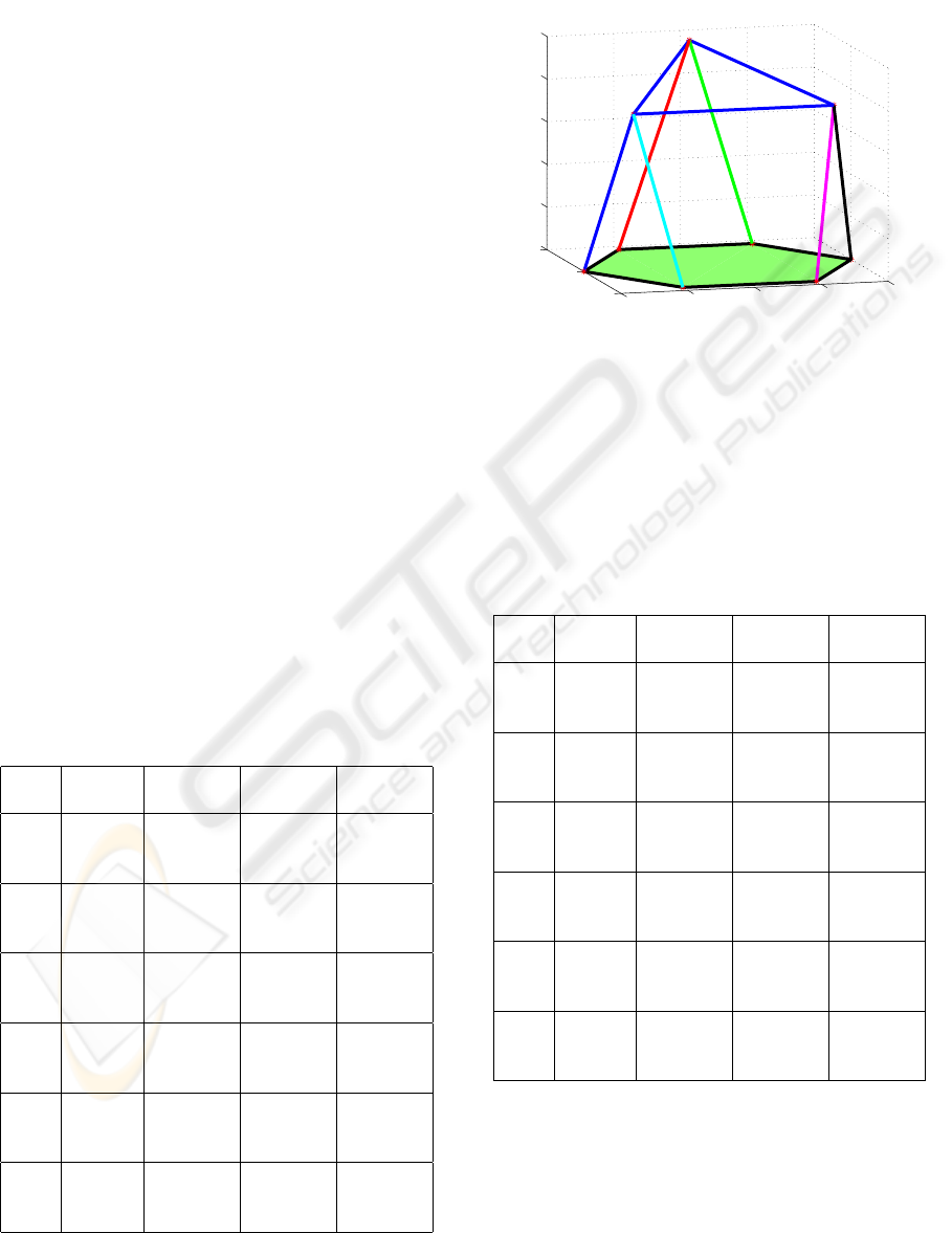
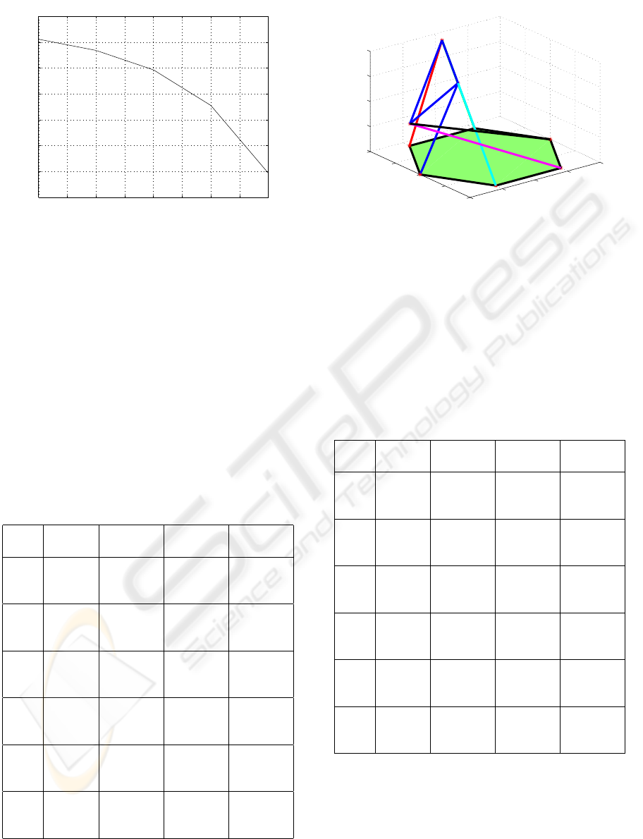
Figure 4 displays the robot at the final configuration
obtained.
−1
−0.5
0
0.5
1
−1
0
1
0
0.5
1
1.5
2
2.5
X
Y
Z
b
1
b
2
b
3
b
4
b
5
b
6
p
1
=p
2
p
3
=p
4
p
5
=p
6
r
1
l
1
r
2
l
2
r
3
l
3
r
4
l
4
r
5
l
5
r
6
l
6
Figure 4: Experiment 1: Final configuration
The algorithm was stopped after 5 iterations, with
a final absolute error of 7.5675 × 10
−11
. Table 3 dis-
plays the lengths of the actuator rods, along with the
corresponding positions of the connecting points in
the P body.
Table 3: Experiment 1: final results
Act. l
i
p
i
b
i
r
i
(0.7500 (0.5000 (0.1250
1 2.0000 -0.4330 -0.8660 0.2165
1.9365) 0.0000) 0.9682)
(0.7500 (1.0000 (-0.1250
2 2.0000 -0.4330 0.0000 -0.2165
1.9365) 0.0000) 0.9682)
(0.0000 (0.5000 (-0.2000
3 2.5000 0.7614 0.8660 -0.0419
2.4473) 0.0000) 0.9789)
(0.0000 (-0.5000 (0.2000
4 2.5000 0.7614 0.8660 -0.0419
2.4473) 0.0000) 0.9789)
(-0.7500 (-1.0000 (0.1250
5 2.0000 -0.4330 0.0000 -0.2165
1.9365) 0.0000) 0.9682)
(-0.7500 (-0.5000 (-0.1250
6 2.0000 -0.4330 -0.8660 0.2165
1.9365) 0.0000) 0.9682)
The key point in this experiment is the fast conver-
gence of the algorithm. Figure 5 illustrates, in loga-
rithmic scale, the evolution of the absolute error.
The solution for the optimal rigid body transforma-
tion is given by the matrix
ICINCO 2005 - ROBOTICS AND AUTOMATION
96

1 1.5 2 2.5 3 3.5 4 4.5 5
10
−12
10
−10
10
−8
10
−6
10
−4
10
−2
10
0
10
2
Temporal evolution of the absolute error in logarithmic scale
Absolute Error in logarithmic scale [m]
Iteration
Figure 5: Experiment 1: Temporal evolution of the
quadratic error
T
final
=
⎡
⎢
⎣
1.0000 0.0000 0.0000 0.0000
0.0000 0.9195 −0.3932 −0.0349
0.0000 0.3932 0.9195 2.1067
0.0000 0.0000 0.0000 1.0000
⎤
⎥
⎦
3.2 Experiment 2
Table 4 presents the values used as initial conditions
by the algorithm for this second experiment. The goal
values for the actuators were set at l
1,...,6
=2.
Table 4: Experiment 2: Initial values
Act. l
i
p
i
b
i
r
i
(0.0000 (0.5000 (-0.2425
1 2.0615 0.8660 -0.8660 0.8402
1.0000) 0.0000) 0.4851)
(0.0000 (1.0000 (-0.6030
2 1.6583 0.8660 0.0000 0.5222
1.0000) 0.0000) 0.6030)
(0.7500 (0.5000 (0.1508
3 1.6583 -0.4330 0.8660 -0.7833
1.0000) 0.0000) 0.6030)
(0.7500 (-0.5000 (0.6063
4 2.0615 -0.4330 0.8660 -0.6301
1.0000) 0.0000) 0.4851)
(-0.7500 (-1.0000 (0.2236
5 1.1180 -0.4330 0.0000 -0.3873
1.0000) 0.0000) 0.8944)
(-0.7500 (-0.5000 (-0.2236
6 1.1180 -0.4330 -0.8660 0.3873
1.0000) 0.0000) 0.8944)
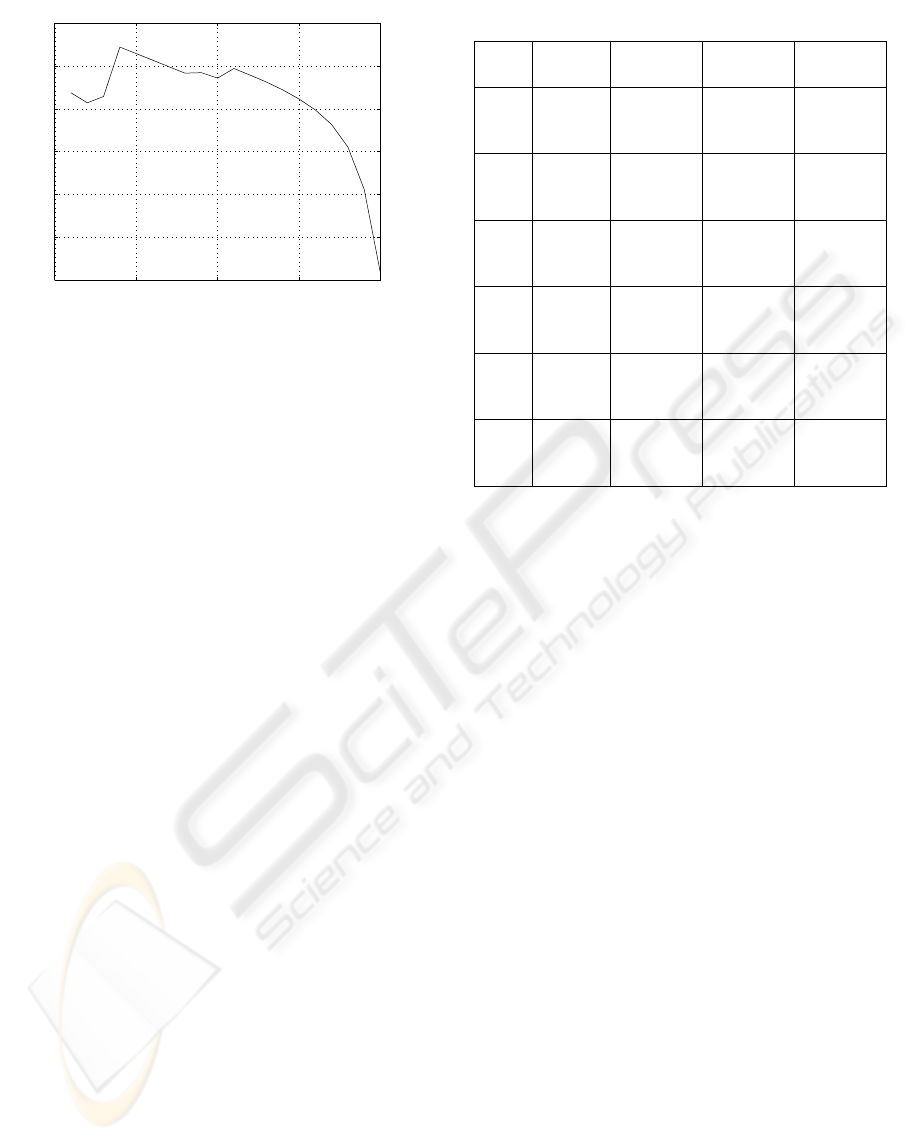
The final robot configuration obtained from this
simulation is presented in Figure 6.
−1
−0.5
0
0.5
1
−1
−0.5
0
0.5
1
0
0.5
1
1.5
2
X
Y
Z
b
1
b
2
b
3
b
4
b
5
b
6
p
1
=p
2
p
3
=p
4
p
5
=p
6
r
1
l
1
r
2
l
2
r
3
l
3
r
6
l
6
r
4
l
4
r
5
l
5
Figure 6: Experiment 2: Final configuration
The algorithm was stopped after 20 iterations, with
a final absolute error of 2.0054 × 10
−8
. Table 5 dis-
plays the lengths of the actuator rods, along with the
corresponding positions of the connecting points in
the P body.
Table 5: Experiment 2: Final values
Act. l
i
p
i
b
i
r
i
(-0.8017 (0.5000 (-0.6509
1 2.0000 0.4629 -0.8660 0.6644
0.7346) 0.0000) 0.3673)
(-0.8017 (1.0000 (-0.9009
2 2.0000 0.4629 0.0000 0.2314
0.7346) 0.0000) 0.3673)
(0.0000 (0.5000 (-0.2500
3 2.0000 0.8660 0.8660 0.0000
1.9365) 0.0000) 0.9682)
(0.0000 (-0.5000 (0.2500
4 2.0000 0.8660 0.8660 0.0000
1.9365) 0.0000) 0.9682)
(-0.7500 (-1.0000 (0.1250
5 2.0000 -0.4330 0.0000 -0.2165
1.9365) 0.0000) 0.9682)
(-0.7500 (-0.5000 (-0.1250
6 2.0000 -0.4330 -0.8660 0.2165
1.9365) 0.0000) 0.9682)
As in the previous experiment, the algorithm con-
verges in an acceptable number of iterations. Figure
7 shows the temporal evolution of the error.
For this experiment, the matrix that corresponds to
the solution of the optimal rigid body transformation
is
KINEMATIC MODELING OF STEWART-GOUGH PLATFORMS
97

0 5 10 15 20
10
−8
10
−6
10
−4
10
−2
10
0
10
2
10
4
Temporal evolution of the absolute error in logarithmic scale
Absolute Error in logarithmic scale [m]
Iteration
Figure 7: Experiment 2: Temporal evolution of the
quadratic error
T
final
=
⎡
⎢
⎣
0.5000 −0.3285 −0.8013 −0.5172
0.8660 0.1897 0.4626 0.2986
0.0000 −0.9253 0.3793 1.5358
0.0000 0.0000 0.0000 1.0000
⎤
⎥
⎦
3.3 Experiment 3
The 6 − 3

/\
3

structure considered in the experi-
ments is known to have 16 real solutions. In general,
these solutions differ significantly from each other.
Therefore, when targeting control applications it is
important to determine the sensitivity of a particular
solution to the initial condition. This is illustrated by
comparing this experiment with experiment 2.
In this experiment the values for the actuator are
set identical to those in experiment 2 but with the ini-
tial position of the P body slightly changed. Table 6
displays the data for this experiment.
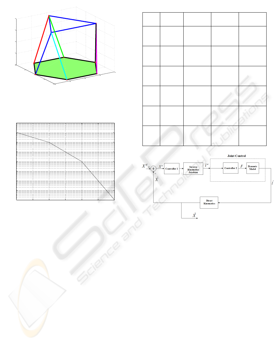
Figure 8 illustrates the final configuration of the ro-
bot which is clearly different from that obtained in
experiment 2.
The algorithm was stopped after 4 iterations, with a
final absolute error of 1.052 × 10
−7
. Table 7 displays
final data obtained in this experiment.
Figure 9 shows the time evolution, in logarithmic
scale, of the error.
For this experiment, optimal rigid body transforma-
tion matrix is given by
T
final
=
⎡
⎢
⎣
1.0000 0.0000 0.0000 0.0000
0.0000 1.0000 0.0000 0.0000
0.0000 0.0000 1.0000 1.9365
0.0000 0.0000 0.0000 1.0000
⎤
⎥
⎦
Table 6: Experiment 3: Initial values
Act. l
i
p
i
b
i
r
i
(0.7500 (0.5000 (0.2236
1 1.1180 -0.4330 -0.8660 0.3873
1.0000) 0.0000) 0.8944)
(0.7500 (1.0000 (-0.2236
2 1.1180 -0.4330 0.0000 -0.3873
1.0000) 0.0000) 0.8944)
(0.0000 (0.5000 (-0.4472
3 1.1180 0.8660 0.8660 -0.0000
1.0000) 0.0000) 0.8944)
(0.0000 (-0.5000 (0.4472
4 1.1180 0.8660 0.8660 -0.0000
1.0000) 0.0000) 0.8944)
(-0.7500 (-1.0000 (0.2236
5 1.1180 -0.4330 0.0000 -0.3873
1.0000) 0.0000) 0.8944)
(-0.7500 (-0.5000 (-0.2236
6 1.1180 -0.4330 -0.8660 0.3873
1.0000) 0.0000) 0.8944)
4 CONCLUSIONS
The paper presents a solution for the direct kinemat-
ics of a Stewart-Gough robot supported on a Newton
method for the search of a rigid body transformation
that places the moving body (the P body in the termi-
nology used in the paper) in a configuration compati-
ble with the desired actuator lengths. The experimen-
tal results show fast convergence to the solution.
4.1 Ongoing work
Experiments 2 and 3 show the importance of the
initial conditions to the final solution. Future work
includes the analysis of solutions sensitivity to initial
conditions.
High performance applications, namely those re-
quiring the manipulation of heavy loads at large band-
widths, require the knowledge of the dynamics model
in order to design the adequate control strategy.
For a large class of applications, e.g., shaking tables
for seismic simulations, the typical frequency band
goes from 0 up to 20-40 Hz (the typical bandwidth
of a real earthquake). Despite the heavy loads consid-
ered in such applications, the bandwith requirements
do not impose detailed knowledge on the dynamics
of the robot. Thus, the use of control schemes us-
ing direct and inverse kinematics solutions obtained
by methods such as the one proposed in this paper are
acceptable.
For the experiments in Section 3, the algorithm
requires less than 20 ms to reach a solution within
the aforementioned errors (Matlab implementation).
ICINCO 2005 - ROBOTICS AND AUTOMATION
98

−1
−0.5
0
0.5
1
−1
−0.5
0
0.5
1
0
0.5
1
1.5
2
X
Y
Z
b
2
b
1
b
3
b
4
b
5
b
6
p
1
=p
2
p
3
=p
4
p
5
=p
6
r
1
l
1
r
2
l
2
r
3
l
3
r
4
l
4
r
5
l
5
r
6
l
6
Figure 8: Experiment 3: Final Robot Solution
1 1.5 2 2.5 3 3.5 4
10
−7
10
−6
10
−5
10
−4
10
−3
10
−2
10
−1
10
0
10
1
Temporal evolution of the absolute error in logarithmic scale
Absolute Error in logarithmic scale [m]
Iteration
Figure 9: Experiment 3: Temporal evolution of the
quadratic error
Therefore, the upper bound on the bandwith is es-
timated at about 25 Hz (assuming that 20 ms cor-
responds to the sample time), this being compatible
with real time control of a shaking table.
Figure 10 illustrates the control strategy under eval-
uation for the shaking table problem. Instead of hav-
ing the inverse kinematics defining the trajectories for
each actuator, this scheme includes both the direct and
inverse kinematics in the control loop. The advantage
of this procedure is that any modeling errors, e.g.,
those due to inaccurate positioning of the actuators
anchor points in the B and P bodies, are compensated
by the control loop.
ACKNOWLEDGEMENTS
This work was supported Programa Operacional So-
ciedade de Informac¸
˜
ao (POSI) in the frame of QCA
III.
Table 7: Experiment 3: Final values
Act. l
i
p
i
b
i
r
i
(0.7500 (0.5000 (0.1250
1 2.0000 -0.4330 -0.8660 0.2165
1.9365) 0.0000) 0.9682)
(0.7500 (1.0000 (-0.1250
2 2.0000 -0.4330 0.0000 -0.2165
1.9365) 0.0000) 0.9682)
(-0.0000 (0.5000 (-0.2500
3 2.0000 0.8660 0.8660 -0.0000
1.9365) 0.0000) 0.9682)
(-0.0000 (-0.5000 (0.2500
4 2.0000 0.8660 0.8660 -0.0000
1.9365) 0.0000) 0.9682)
(-0.7500 (-1.0000 (0.1250
5 2.0000 -0.4330 0.0000 -0.2165
1.9365) 0.0000) 0.9682)
(-0.7500 (-0.5000 (-0.1250
6 2.0000 -0.4330 -0.8660 0.2165
1.9365) 0.0000) 0.9682)
Figure 10: Control architecture
REFERENCES
Dietmaier, P. (1998). The stewart-gough platform of gen-
eral geometry can have 40 real postures. Advances in
Robot Kinematics: Analysis and Control, pages 1–10.
Hopkins, Brian R., W. I. R. L. (2002). Modified 6-psu
platform. Industrial Robot: An International Journal,
29(5):443–451.
Jakobovi
´
c, D. and Budin, L. (2002). Forward kinemat-
ics of a stewart parallel mechanism. pages 149–154.
Opatija, May 26-28.
Khalil, W. and S., G. (2004). Inverse and direct dynamic
modeling of gough-stewart robots. IEEE Trans. on
Robotics, 20(4):754–762.
Merlet, J. (2000). Parallel Robots. Kluwer Academic.
Parikh, P. and Lam, S. (2005). A hybrid strategy to solve the
forward kinematics problem in parallel manipulators.
IEEE Transactions on Robotics, 21(1):18–25.
KINEMATIC MODELING OF STEWART-GOUGH PLATFORMS
99