
APPLICATION OF DE STRATEGY AND NEURAL NETWORK
In position control of a flexible servohydraulic system
Hassan Yousefi, Heikki Handroos
Institute of Mechatronics and virtual Engineering, Mechanical Engineering Department,
Lappeenranta University of Technology, 53851,Lappeenranta, Finland
Keywords: Differential Evolution, Backpropagation, Position Control, Servo-Hydraulic, Flexible load.
Abstract: One of the most promising novel evolutionary algorithms is the Differential Evolution (DE) algorithm for
solving global optimization problems with continuous parameters. In this article the Differential Evolution
algorithm is proposed for handling nonlinear constraint functions to find the best initial weights of neural
networks. The highly non-linear behaviour of servo-hydraulic systems makes them idea subjects for
applying different types of sophisticated controllers. The aim of this paper is position control of a flexible
servo-hydraulic system by using back propagation algorithm. The poor performance of initial training of
back propagation motivated to apply the DE algorithm to find the initial weights with global minimum. This
study is concerned with a second order model reference adaptive position control of a servo-hydraulic
system using two artificial neural networks. One neural network as an acceleration feedback and another
one as a gain scheduling of a proportional controller are proposed. The results suggest that if the numbers of
hidden layers and neurons as well as the initial weights of neural networks are chosen well, they improve all
performance evaluation criteria in hydraulic systems.
1 INTRODUCTION
Problems which involve global optimization over
continuous spaces are ubiquitous throughout the
scientific community. In general, the task is to
optimize certain properties of a system by
pertinently choosing the system parameters. For
convenience, a system’s parameters are usually
represented as a vector. The standard approach to an
optimization problem begins by designing an
objective function that can model the problem’s
objectives while incorporating any constraints.
Consequently, we will only concern ourselves
with optimization methods that use an objective
function. In most cases, the objective function
defines the optimization problem as a minimization
task. To this end, the following investigation is
further restricted to minimization problems. For
such problems, the objective function is more
accurately called a “cost” function.
One of the most promising novel evolutionary
algorithms is the Differential Evolution (DE)
algorithm for solving global optimization problems
with continuous parameters. The DE was first
introduced a few years ago by Storn (Storn, 1995)
and Schwefel (Schwefel, 1995).
When the cost function is nonlinear and non-
differentiable Central to every direct search method
is a strategy that generates variations of the
parameter vectors. Once a variation is generated, a
decision must then be made whether or not to accept
the newly derived parameters. Most stand and direct
search methods use the greedy criterion to make this
decision. Under the greedy criterion, a new
parameter vector is accepted if and only if it reduces
the value of the cost function.
The extensive application areas of DE are
testimony to the simplicity and robustness that have
fostered their widespread acceptance and rapid
growth in the research community. In 1998, DE was
mostly applied to scientific applications involving
curve fitting, for example fitting a non-linear
function to photoemissions data (Cafolla AA.,
1998). DE enthusiasts then hybridized it with
Neural Networks and Fuzzy Logic (Schmitz GPJ,
Aldrich C., 1998) to enhance or extend its
performance. In 1999 DE was applied to problems
involving multiple criteria as a spreadsheet solver
application (Bergey PK., 1999). New areas of
interest also emerged, such as: heat transfer (Babu
BV, Sastry KKN., 1999), and constraint satisfaction
problems (Storn R., 1999) to name only a few. In
133
Yousefi H. and Handroos H. (2005).
APPLICATION OF DE STRATEGY AND NEURAL NETWORK - In position control of a flexible servohydraulic system.
In Proceedings of the Second International Conference on Informatics in Control, Automation and Robotics, pages 133-140
DOI: 10.5220/0001190301330140
Copyright
c
SciTePress
2000, the popularity of DE continued to grow in
areas of electrical power distribution (Chang TT,
Chang HC., 2000), and magnetics (Stumberger G. et
al, 2000). 2001 furthered extensions of DE in areas
of environmental science (Booty WG et al, 2000),
and linear system models (Cheng SL, Hwang C.,
2001). By the year 2002, DE penetrated the field of
medical science (Abbass HA., 2002). Most recently
in 2003, there has been a resurgence of interest in
applying DE to problems involving multiple criteria
(Babu BV, Jehan MML. 2003).
Electro-hydraulic servomechanisms are known
for their fast dynamic response, high power-inertia
ratio and control accuracy. In the fluid power area,
neural network systems have been used for control,
identification and modeling of the system (Chen,
1992). The popularity of neural networks can be
attributed, in part, to their ability to deal with non-
linear systems. In addition, a neural network
approach uses a parallel distributed processing
concept
(D.E.Rumelhart, et al, 1986). It has the
capability of improving its performance through a
dynamic learning process and, thus, provides
powerful adaptation ability. Since neural networks
are fashioned after their human neural counterparts,
they can be ‘trained’ to do a specific job by
exposing the networks to a selected set of input–
output patterns. A comparatively convenient
method is to have a reference response model,
which can be the tracking object of the control
system. Following the model reference adaptive
control theory (Franklin, 1984), an adaptive
reference model is used in this study and
implemented in the microcomputer to control a
hydraulic variable motor.
Gain scheduling based on the measurements of
the operation conditions of the process is often a
good way to compensate for variations in the
process parameters or the known nonlinearities of
the process.
The main aim of the following study is to apply
the DE strategy to find the best initial weights of the
proposed neural networks to improve the
performance of position tracking of the reference
model.
The structure of the paper is the following: in
section 2 description of the flexible servo-hydraulic
system, section 3 controller design, section 4
differential evolution algorithm, section 5 presents
the main results of this work, and section 6 draws
conclusions.
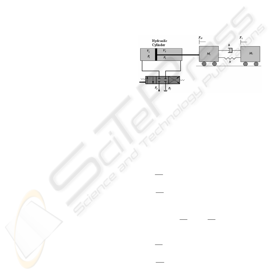
2 SERVO HYDRAULIC SYSTEM
The hydraulic system with flexible load shown in
figure 1 is comprised of a servo-valve, a hydraulic
cylinder and two masses that are connected by a
parallel combination of spring and damper. The
schematic diagram of the system is illustrated in
figure1.
The nonlinearity of the constitutive equations as
well as the sensitivity of the system’s parameters to
the sign of the voltage fed to the valve make the
control of system too complicated (Viersma, 1980).
2.1 System Model
Figure 1: Schematic Diagram of System.
Applying Newton’s second law for each mass
without consideration of coulomb friction results,
2211
211
)()(
ApAp
XXkXXbXbXm
lplppp
−+
−−−−−=
&&&&&
)()(
plpL2l2
XXkXXbXm −−−−=
&&&&
(1, 2)
Continuity equations for the output ports of the
servo valve results,
⎪
⎪
⎩
⎪
⎪
⎨
⎧
+−=
−=
)(
)(
22
2
2
11
1
1
p
e
p
e
XAQ
V
p
XAQ
V
p
&
&
&
&
β
β
(3)
Introducing two new parameters,
1
C and
2
C ,
defined as,
e
1
1
V
C
β
= ,
e
2
V
2C
β
=
Equation 3 can be written in the form of,
⎪
⎪
⎩
⎪
⎪
⎨
⎧
+−=
−=
)(
1
)(
1
22
2
2
11
1
1
p
p
XAQ
C
p
XAQ
C
p
&
&
&
&
(4)
The volumes between the valve and each side of
piston are calculated as,
01p11
XAV
ν
+
=
02p22
XLAV
ν
+
−
=
)(
ICINCO 2005 - INTELLIGENT CONTROL SYSTEMS AND OPTIMIZATION
134
If the tank pressure is set to equal to zero (
0
=
T
p ),
the nonlinear equations of flow rate of valve can be
written in the simplest form, as follow,
⎪
⎩
⎪
⎨
⎧
≥−
=
0u puc
0u ppuc
Q
1v
1sv
1
p
(5)
⎪
⎩
⎪
⎨
⎧
−
≥
=
0u ppuc
0u puc
Q
2sv
2v
2
p
(6)
Table 1: Setup Parameters
Kg 278m
1
=
m
1L =
Kg 110m
2
=
m
Ns
1000b
1
=
24
1
m10048A
−
×= .
m
Ns
500b
2
=
24
2
m10244A
−
×= .
Pa
8
e
104 ×=
β
m
N
136670k =
Mpa14P
s
=
34
01
m10132
−
×= .
ν
3
m
4
02
1007.1
−
×=
ν
)(sVPa
m
102
2
1
3
8−
×=
v
c
Where,
nn
n
v
pu
Q
c
∆
=
The setup parameters of system are shown in
Table1.
Following, the structure of controller for
positioning control of each mass is proposed.
3 CONTROLLER DESIGN
Here, the aim of the controller is position tracking
of a reference model. Classical approaches, like P or
PD regulators for positioning of hydraulic drives, do
not give satisfactory performance. For this reason,
adaptive control techniques, adaptive reference
model, and gain scheduling are used to improve the
performance of Controller (4). The variations of
parameters depending on the change in the sign of
voltage fed to the valve are compensated by gain
scheduling block. The second neural network is
impelled to improve the lack of damping in
hydraulic systems. Following the reference model
and each neural network are proposed.
3.1 Reference Model
The desire linear, second order, reference model
was selected to run parallel with the nonlinear
system. The natural frequency,
n
ω
, of this model set
equal to as 7 rad/sec with the damping ratio,
ζ
, of
0.9.
2
nn
2
2
n
ref
s2s
sG
ωζω
ω
++
=
)( (7)
There are kinds of method to find a reference
model such as ITAE or Bessel transfer functions.
The Bessel transfer functions have not overshot
when
n
ω
is equal to one, but when
n
ω
is greater
than one the overshot appears.
The natural frequency of system was chosen in a
manner that the response of system is as fast as
possible. The chosen damping ratio provides the
minimum overshoot of reference model.
3.2 Neural Network Design
Basic neural networks consist of Neurons, weights
and activation function. The weights are adapted to
achieve mapping between the input and output sets
in the manner to track reference model. Many
neural networks are successfully used for various
control applications. In this study the
backpropagation algorithm with momentum term
was used to update the weights and biases of neural
network (Rumelhart, 1986). The backpropagation
algorithm is a learning scheme in which the error is
backpropagated layer by layer and used to update
the weights. The algorithm is a gradient descent
method that minimizes the error between the desired
outputs and the actual outputs calculated by the
MLP.
The backpropagation training process requires
that the activation functions be bounded,
differentiable functions. One of the most commonly
used functions satisfying these requirements is the
hyperbolic tangent function. This function has a
monotonic increasing in the range of –1 to 1. The
mathematical model of hyperbolic tangent can be
written in the form of,
xx
xx
ee
ee
xf
−
−
+
−
=
)( (8)
The learning procedure requires only that the
change in weights and biases are proportional to the
wE
p
∂
∂
/ . True gradient descent requires that
infinitesimal steps be taken. The constant of
proportionality is the learning rate in the procedure.
The bigger change of this constant, the bigger
change in the weights. For practical purposes we
APPLICATION OF DE STRATEGY AND NEURAL NETWORK - In position control of a flexible servohydraulic system
135
choose a learning rate that is as large as possible
without exciting oscillation. This offers the most
rapid learning. One way to increase the learning rate
without leading to oscillation is to modify the
general delta rule to include a momentum term. This
can be accomplished by the following rule,
)()()( nwo1nw
jipipjji
∆+=+∆
α
δ
η
(9)
where n indicates the presentation number. The
parameter of
η
is the learning rate, and
α
is a
constant which determines the effect of past
changes on the current direction of movement in
weight space.
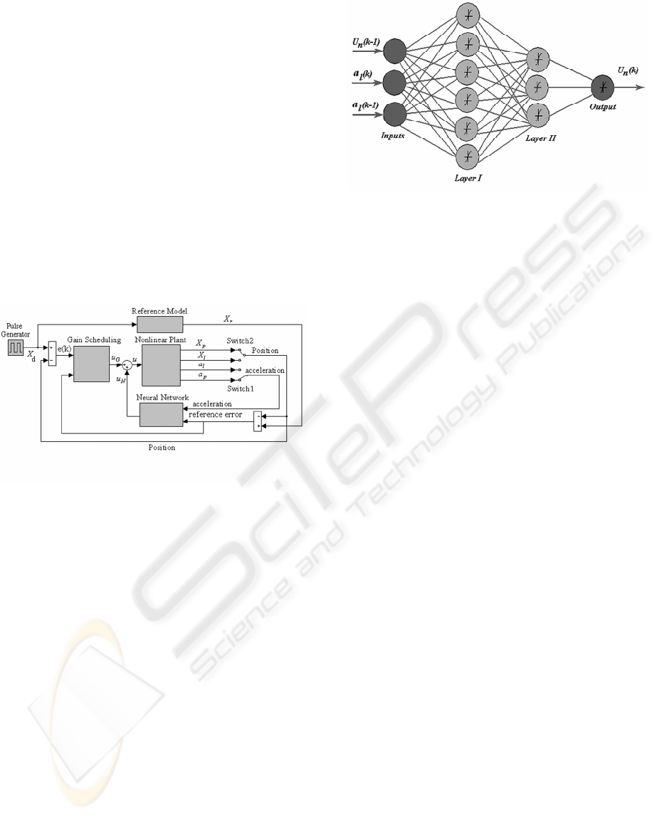
The proposed controller depicted in figure 2,
composed of two neural networks, shown as blocks
Neural Networks and Gain Scheduling. Neural
Network Block is used as acceleration feed back to
improve the dynamic behavior of system (lack of
damping).
Figure 2: Schematic Diagram of Neural Controller
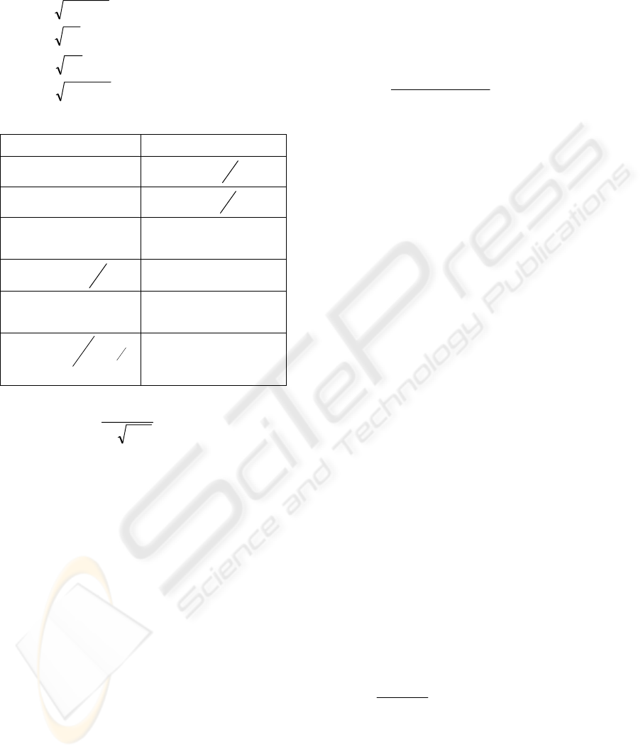
Neural networks parameters are updated online by
learning rate and momentum factors. As it shown in
figure, the proposed neural network has two hidden
layers, figure3, one input and one output layer. The
inputs of neural network are two accelerations
( )(ka
i
, )( 1ka
i
− ) and the output of pervious
step, )1( −ku
n
. Several kinds of structure with one
or three hidden layers were tested. The proposed
structure has this ability to emulate the acceleration
feedback and improve the dynamic behavior of
system.
The second neural network, gain scheduling
network, has the same structure as pervious one, but
the inputs are the two controller errors (
)(ke ,
)( 1ke − ) and the output of last step, )( 1ku
G
−
.
Due to the poor results of p-controller in return
stage the second neural network tried to compensate
this matter. Finally, the controller output,
summation of
N
u and
G
u , is fed to the system.
Choosing the initial weights are too important in
back-propagation algorithm. To avoid local minima
problem, the genetic algorithm is used to find the
off-line weights (Corne. 1999).
Figure 3: Structure of Neural Network
For online training with backpropagation algorithm
the learning rate of
6
102
−
×=
η
and 00010.=
α
are
used. The simulation results are depicted in result
section.
Following the results of using new controller is
compared with common p-controller.
4 DE STRATEGY
Differential evolution (DE) is a simple yet powerful
population based, direct-search algorithm for
globally optimizing functions defined on totally
ordered spaces, including especially functions with
real-valued parameters. Real parameter optimization
comprises a large and important class of practical
problems in science and engineering.
There are two variants of DE that have been
reported, DE/rand/1/bin and DE/best/2/bin. The
different variants are classified using the following
notation:
DE
/x /y/z;
where
• x indicates the method for selecting the
parent chromosome that will form the base
of the mutated vector. Thus, DE
/rand/y/z
selects the target parent in a purely random
manner. In contrast, DE
/best/y/z selects the
best member of the population to form the
base of the mutated chromosome.
• y indicates the number of difference
vectors used to perturb the base
chromosome.
• z indicates the crossover mechanism used
to create the child population. The
bin
acronym indicates that crossover is
controlled by a series of independent
binomial experiments.
Following, the schematic procedure of a class of DE
( DE/rand/1/bin) is presented.
ICINCO 2005 - INTELLIGENT CONTROL SYSTEMS AND OPTIMIZATION
136
()
[]
)((lo)
max
,x:bounds initial
and 1,0CR , 1,0F ,4,G D,
:
hi
x
NP
Input
∈+∈≥
D= number of parameters.
NP= population size.
F=scale factor.
CR= crossover control constant.
G
max
=Maximum number of generation.
hi, lo= upper and lower initial parameter bounds,
respectively.
[]
()
⎪
⎩
⎪
⎨
⎧
−+=
≤∀∧≤∀
=
)((hi)
j
)(
,
oGi,j,
x. 1,0x
:Dj NPi
:
lo
j
lo
ij
xrandx
Initialize
(11)
: NPi
GG While
max
≤∀
p
{}
()
[
)
⎪
⎪
⎪
⎪
⎪
⎪
⎪
⎪
⎩
⎪
⎪
⎪
⎪
⎪
⎪
⎪
⎪
⎨
⎧
⎪
⎩
⎪
⎨
⎧
≤
=
⎪
⎪
⎩
⎪
⎪
⎨
⎧
=∨
−+
=
≤∀
≠≠≠
∈
++
+
+
otherwise
)()F(u if
:
otherwise
)jj 1,0(rand If
.
u
: Dj
ieach once selectedrandon j
irrr :except
selectedrandomly ,,...,2,1,,r
:ionRecombinat and Mutate
,
,1Gi,1,
1,
,,
rj
,,,,,,
1Gj,i,
r
321
321
213
Gi
GiGi
Gi
Gij
GrjGrjGrj
x
xFu
x
Select
x
CR
xxFx
NPrr
p
(12)
1+= GG (13)
The aforementioned algorithm finds the global
minima more reliable than the other methods. Note
that these kinds of algorithms are useful in off-line
training as the speed of approaching in not fast.
Here, the numbers of initial weights for each neural
network are 49. Following is the selected
parameters for this strategy,
D= 49,
NP=5
× 49 ≈ 250,
F=0.8,
CR=0.7,
The initial upper and lower bounds are 1,-1,
respectively.
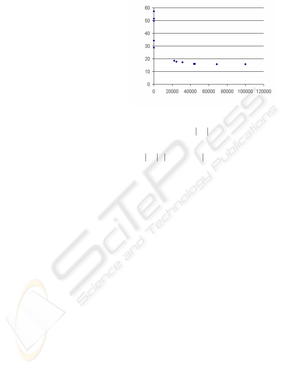
The results show that DE can find the global
minimal cost for the system. Depend on the
expected value of cost, the DE will find the proper
weights. Here the cost of system is defined as
follow,
Figure 4: Cost of System against the Number of its
Iterations
∑
=
=
=
2000
1
,
)()(
K
k
Gi
kexF (14)
Where,
)()()( kXkXke
lr
−= (15)
The desire input (
d
X ) is pulse input with the
amplitude of 0.3 (m) and period of 4 (sec.). In the
first step the weights of neural network compensator
were found. To do that, the gain scheduling was
replaced with a constant around 5 and then the cost
for half of period was calculated. The sampling time
here is one millisecond, so the cost will be
calculated 2000 times in each iteration.
Figure 4 shows the amount of cost against its
iteration number. The result indicates that at the
earlier iteration the amount of cost is too big. Also
the algorithm finds new child generations with
lower cost to fast (cost bigger than 30). To find the
lower cost, the number of iterations must growth up.
As it shown, when the number of iteration is around
30000, the related cost is around 17.6, after around
34000 iterations the cost will be fixed at 15.6. This
cost will be constant and its related weights has the
global minimum cost for the proposed neural
compensator.
After aforementioned step for tuning the neural
network, using the same strategy, the weights of
neural gain scheduling will be found.
In the next section the proposed neural networks
will be impelled to position controlling of the
system. The important factor in DE is factor of F.
The iteration number is incredibly related to this
factor. However, the change of crossover factor has
not essential effect in decreasing the number of
iterations. The chosen value is recommended in
many cases to be useful. In this study, the number
of generation was 1973 times during 100000
iterations.
APPLICATION OF DE STRATEGY AND NEURAL NETWORK - In position control of a flexible servohydraulic system
137
5 RESULTS AND DISCUSSIONS
In this section the results of using proposed
controller for two cases are provided. These
controllers are tracking the reference model for
piston tracking (
1
m ), case I, and flexible load
tracking (
2
m ), case II, respectively.
The desire input (
d
X ) is pulse input with the
amplitude of 0.3 (m) and period of 4 (sec.).
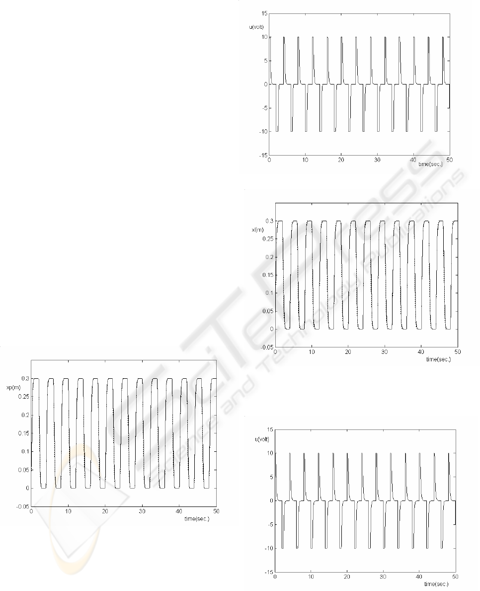
5.1 Piston Tracking
Figure 5 is the piston tracking of the reference
model using neural network with gain scheduling.
Figure 6 is its controller effort that will be fed to
nonlinear system.
The maximum and minimum voltages fed to the
valve are limited to
10± (Volt). As it shown in
figure 6, the maximum and minimum of voltage are
banded because of valve restriction.
5.2 Fexible Load Tracking
In this section the results of using second controller
to track of reference model for flexible load is
presented. Figure 7 is the flexible load tracking of
the reference model using neural network with gain
scheduling.
Figure 5: Result of Mass Load Tracking Using Neural
Network with Gain Scheduling. The Solid Line Shows the
Reference Model and Dots Line Show Mass Load
Position
Figure 6: Controller Effort Using Neural Controller with
Neural Gain Scheduling
Figure 7: Simulation Result of Flexible Load Tracking
Using Neural Network with Gain Scheduling. The Solid
Line Shows the Reference Model and Dots Line Show
Mass Load Position.
Figure 8: Controller Effort Using Neural Controller with
Gain Scheduling
ICINCO 2005 - INTELLIGENT CONTROL SYSTEMS AND OPTIMIZATION
138

Figure 8 is its controller effort that will be fed to the
system.
The acceleration of flexible load is used for the
neural network block. The results are satisfactory
and illustrate the capability of the neural network in
controlling and compensating the dynamic of the
servo hydraulic systems.
As it was shown in the figure 5, in rising and
falling stages, the flexible load tracking is similar to
that of the piston tracking.
Figure 7 shows that the neural network with the
gain scheduling has very good performances during
the rising and falling. The aforementioned controller
can track the reference model very well. Figure 8
shows the output of controller is smooth and has not
any oscillation.
6 CONCLUSIONS
In the present paper the application of DE and back-
propagation algorithm in position control of a
flexible servo-hydraulic system was studied. The
results suggest that neural network has good
performance if the initial weights of system are set
correctly. To avoid the local minima, Differential
Evolution Algorithm is essential. These kinds of
algorithms are too slow, so they are useful only in
off-line training.
In this article the Differential Evolution
Algorithm for handling multiple nonlinear functions
was proposed and demonstrated with a set of two
difficult test problems. With all test cases, the
algorithm demonstrated excellent effectiveness,
efficiency and robustness. The architectures and the
number of hidden layers are the other essential keys
to have a well-performed neural network. If the
number of hidden layers or neurons in each layer is
not enough the results will be poor. Several
structures were tested and the aforementioned
architecture was adapted.
In light of above, using neural network to
compensate the dynamic of hydraulic systems is an
essential factor to improve their performances.
Also, the implementing of the gain scheduling
overcomes the variations of parameters during its
perform.
7 NOMENCHLACHERS
1
A piston area in chamber one
2
A piston area in chamber two
i
B biases (
i
=1, 2, 3)
0
b viscous friction coefficients of cylinder
1
b viscous friction coefficient of flexible load
v
c flow coefficient
k spring constant
p
k proportional gain
L stroke
1
m mass of rigid body
2
m mass of flexible load
1
p pressure in chamber one
2
p pressure in chamber two
s
p pressure supply
T
p tank pressure
1
Q flow rate in chamber one
2
Q flow rate in chamber two
n
Q nominal flow
u
control signal
1
u proportional controller signal
2
u neural network controller signal
n
u nominal controller signal
1
V compressed volume of chamber one
2
V compressed volume of chamber two
ji
w neural network weights ( i =1,2,3)
l
x load position
p
x piston position
r
x reference position
d
X desire position
n
p
∆
nominal pressure difference
α
momentum rate
e
β
effective bulk modulus
η
learning rate
0
ν
volume of pipe between valve and cylinder
port
n
ω
natural frequency
REFERENCES
Abbass HA., 2002. An Evolutionary Artificial Neural
Networks Approach for Breast Cancer Diagnosis.
Artificial Intelligence in Medicine, 25, 265–281.
Babu BV, Jehan MML. 2003. Differential Evolution for
Multi-Objective Optimization. Proceedings of 2003
Conference on Evolutionary Computation (CEC-
2003), Canberra, Australia, 2696–703.
APPLICATION OF DE STRATEGY AND NEURAL NETWORK - In position control of a flexible servohydraulic system
139

Babu BV, Sastry KKN., 1999. Estimation of Heat Transfer
Parameters in a Trickle-Bed Reactor Using
Differential Evolution and Orthogonal Collocation.
Computers and Chemical Engineering, 23(3), 327–
339.
Bergey PK., 1999. An Agent enhanced Intelligent
Spreadsheet Solver for Multi-Criteria Decision
Making. Proceedings of AIS AMCIS 1999: Americas
Conference on Information Systems, Milwaukee, USA,
966–8.
Booty WG, D Lam CL, Wong IWS, Siconolfi P., 2000.
Design and Implementation of an Environmental
Decision Support System. Environmental Modeling
and Software, 16(5), 453–458.
Cafolla AA., 1998. A New Stochastic Optimization
Strategy for Quantitative Analysis of Core Level
Photoemission Data. Surface Science, 402–404,561–
565.
Chang TT, Chang HC., 2000. An Efficient Approach for
Reducing Harmonic Voltage Distortion in
Distribution Systems with Active Power Line
Conditioners. IEEE Transactions on Power Delivery,
15(3), 990–995.
Chen, S. and Billings, S. A., 1992. Neural Networks for
Dynamical System Modeling and Identification. Int.
J. Control, 56(2), 319-346.
Cheng SL, Hwang C., 2001. Optimal Approximation of
Linear Systems by a Differential Evolution
Algorithm. IEEE Transactions on Systems, Man and
Cybernetics, Part A, 31(6), 698–707.
David Corne, Marco Dorigo and Fred Glover, 1999, The
book. New Ideas in Optimization, McGraw-Hill.
D.E.Rumelhart, et al, 1986. Learning Internal
Representations: by Error Propagation. Parallel
Distributed Processing Explorations in the
Microstructures of Cognition, 1,318-362.
Gene F. Franklin, et al., 1986, The Book. Feedback
Control of Dynamic Systems, Addison-Wesley.
Schmitz GPJ, Aldrich C., 1998. Neuro-Fuzzy Modeling
of Chemical Process Systems with Ellipsoidal Radial
Basis Function Neural Networks and Genetic
Algorithms. Computers & Chemical Engineering, 22,
1001–1004.
Schwefel, H.P., 1995, The Book, Evolution and Optimum
Seeking, John Wiley.
Storn R., 1999. System Design by Constraint Adaptation
and Differential Evolution. IEEE Transactions on
Evolutionary Computation, 3(1), 22–34.
Storn, R. and Price, K.V.,1995. Differential evolution - a
Simple and Efficient Adaptive Scheme for Global
Optimization over Continuous Spaces, Technical
Report TR-95-012, ICSI.
Stumberger G, Pahner U, Hameyer K., 2000.
Optimization of Radial Active Magnetic Bearings
Using the Finite Element Technique and the
Differential Evolution Algorithm. IEEE Transactions
on Magnetics, 36(4), 1009–13.
Taco J. Viersma, 1980, The Book. An analysis, Synthesis
and Design of Hydraulic Servosystems and Pipelines,
Elsevier.
ICINCO 2005 - INTELLIGENT CONTROL SYSTEMS AND OPTIMIZATION
140
