
Characterising Evoked Potential Signals Using Wavelet
Transform Singularity Detection
Conor McCooey
1
and Dinesh Kant Kumar
1
1
School of Electrical & Computer Engineering, RMIT University, PO Box 2476V,
Melbourne,VIC 3000, Australia
Abstract: A new method of viewing evoked potential data is described. This
method, called the peak detection method, is based on singularity detection
using the discrete wavelet transform. The peaks and troughs of an EEG
recording are identified and characterized using the algorithms of this method,
resulting in a linear decomposition of the data into sets of individual peaks.
Then, by classifying the peaks in terms of latency (time), magnitude (voltage
potential) and width (scale), the locations of higher concentrations of similar
peaks are identified. These are grouped and sub-averaged, yielding sets of sub-
averaged peaks that characterize the shape and give a measure of the
repeatability of particular sub-averages within the visual evoked potential
ensemble average signal. This method highlights evoked potential features that
may be obscured or cancelled out with standard ensemble averaging. This is
demonstrated for visual evoked potential data taken from a single subject.
1 Introduction
Electroencephalography (EEG) is the electrical recording of brain activity and is
generated by the summation of spatially and temporally separated action potentials. It
is a complex signal and even though it appears noisy, is very useful for identifying
certain brain conditions. For many years the frequency spectrum of EEG has been
examined and usefully interpreted for clinical and research purposes.
The Fourier transform uses time invariant sine waves and effectively gives a
measure of the presence of a particular range of frequencies of a given time course
signal. In the process of performing the transform the time location of the frequency
is lost. The wavelet transform [1] uses time bound waves (wavelets) and may be
thought of as an extension of the Fourier transform where the frequency content and
time location are recorded simultaneously. Wavelet representations are more efficient
than the traditional Fourier representation where the signal is non-stationary such as
EEG. Such a method is able to localize the time when changes in the signal properties
occur.
Evoked Potentials (EPs) are EEG recordings in response to visual, auditory or
somatosensory sensory stimulation. EPs are used by clinicians to study specific
neurological disorders. Due to the presence of background activity and noise, a single
stimulus response is not detectable because the signal of interest is embedded in
similar-sized or larger ongoing background EEG signals and so multiple stimuli
McCooey C. and Kant Kumar D. (2005).
Characterising Evoked Potential Signals Using Wavelet Transform Singularity Detection.
In Proceedings of the 1st International Workshop on Biosignal Processing and Classification, pages 3-11
DOI: 10.5220/0001191700030011
Copyright
c
SciTePress

triggered recordings are taken. Typically, ensemble averaging is used to detect the
Evoked Potential and in the case of visual evoked potentials (VEP) requires 100 to
200 repeats of the stimulus to obtain an observable response. Averaging of these
epochs reduces the uncorrelated background EEG signals which tends towards a zero
level as it is considered random in nature, while the stimulus response is time-locked
to the stimulus and so averages to a particular voltage profile.
If the EP recording consisted purely of the time-locked stimulus response and the
background activity was purely Gaussian in nature, then there would exist a high
degree of repeatability across sequential tests on individual subjects. Experience
under such conditions shows that, while strong similarities show through the EP,
significant variations from one test to the next are observed.
Obtaining single-trial evoked potential reconstruction would greatly assist in
addressing some of the unanswered questions regarding evoked potential activity.
Researchers have attempted to develop several methods to discern the sought-after
signal from the background activity. These include time-frequency digital filtering
[2], Matched Filtering [3], Wavelet Denoising [4] and Wavelet Thresholding.
One important property of EEG recordings is the presence of singularities and
peaks. EEG signals are characterized by sharp, irregular non-stationary transitions,
which are known as singularities [5]. The singularities of EEG have been investigated
using a different method called fragmentary decomposition [6] with the same goal of
eliciting a better understanding of the EEG recording using discrete peaks.
This research aims to determine the singularity features of EEG recordings in order
to overcome some of the limitations in the analysis of evoked potentials by averaging.
This paper describes a method where the singularities are grouped together to identify
the individual peaks that are the basic building block of the EEG recordings.
2 Theory
A wavelet is a time domain wave which is localized, oscillatory and with zero
average. A wavelet, ψ(t) may be expressed in terms of a scale or dilation factor, s,
which as it is varies compresses or expands the wavelet shape and a translation factor,
u that shifts the wavelet along the time axis. Wavelets have narrow time and
frequency support (ideally) and are suitable for singularity identification and peak
detection.
The output of the wavelet transform is a set of coefficients along the time axis for
each scale factor [7]. These coefficients indicate the correlation between the signal
and the wavelet at the specific scale and translation. These are larger when the signal
at the temporal location of the wavelet has spectral properties similar to the wavelet
scale.
One practical implementation of the dyadic wavelet transform uses a filter bank
algorithm and a dyadic scale (2
j
) and is called the “algorithme à trous” [5]. It
generates a detail component (similar to a low pass filter) at each 2
j
scale up to the
maximum calculated scale, together with a remaining approximation component. By
selecting the wavelet function to be the derivative of a smoothing function, such as
the quadratic spline wavelet of degree 2, the evolution of the local maxima of the
wavelet transform modulus across scales can be used to detect local singularities. The
4

detail components, taken from the “algorithme à trous” method, yield a set of
coefficients for each scale.
By selecting only the modulus maxima values that fitted a linear relationship
across scales, a large set of wavelet coefficients may be simplified into a much
smaller discrete set of coefficients grouped per singularity [5]. This is a powerful step
forward in the characterization of a signal into a group of singularities. An inverse
discrete wavelet transform algorithm that gives a good estimate of the original signal
has also been demonstrated [5].
The technique reported in this paper detects singularities using the Discrete
Wavelet Transform (DWT). Singularities are grouped into peaks within the signal and
the EEG recording is decomposed into a linearly independent set of peaks that sum to
approximate the original signal.
Once identified, each peak is then described by its characterizing features - time
latency, width of peak and height of peak and then classified using these properties to
populate a multi-dimensional matrix. Performed across all peaks and all epochs for
the full EEG recording, this allows areas of local concentration to be identified. This
local activity may then be extracted and sub-averaged to yield a localized EP signal.
This paper demonstrates that the concentration matrices used in conjunction with the
ensemble averaging may be used to decompose the EP peaks.
This paper reports the use of the technique for flash visual evoked potentials
(VEP). This could be extended to other stimulation techniques. Other possible
applications include denoising, data compression and all applications where non-
stationary signal activity is important.
3 Method
3.1 Peak Detection
Singularity detection using the DWT [5] is the starting point for the theory outlined in
this paper. Singularities characterize areas of large magnitude change in the signal
over a short period i.e. points where there is a large slope. A peak may be thought of
as a pair (or triplet) of singularities that record a simple shift away from and back to a
particular baseline. These singularity coefficient sets are matched into pairs (or
triplets) that identify distinct peaks within the data. The position and value of both the
detail and approximation components are recorded in a single line of an array for each
singularity. Using these arrays, sets of singularities are made that would combine to
make peaks using a set of guidelines listed below:
(a) A pair of singularities is more likely to form a peak if the absolute magnitudes of
the detail components at the highest scale level for each singularity are similar to one
another.
(b) Singularities that increase with time have positive coefficients and those that
decrease with time have negative coefficients. Therefore a peak must be made up of
both positive and negative coefficient singularities.
(c) Singularities that match to form a peak have similar maximum detail scale (s)
level within ±1 scale factor of each other.
5

(d) The gap between the position of the first detail component of each singularity in a
pair is related to the dyadic scale factor and fits the rule in equation (1) where p
1
(g
x
)
represents the first coefficient value for singularity (g
x
) and x is a sequential list of
identified singularities.
2
s
< p
1
(g
2
) – p
1
(g
1
) < 2
s+1
. (1)
The PDM algorithm matches the singularities to generate singularity sets governed
by the above guidelines. Using the inverse DWT and only the coefficients of each
singularity set, a signal representation for each identified peak is generated. These
peaks are added together, in the time domain, to yield a close approximation of the
original signal. All peaks are defined as starting at the zero baseline, deviating either
positively or negatively and returning to the baseline. Bi-phasic peaks are divided
into 2 mono-phasic peaks – one positive and one negative. The features of all the
detected peaks are identified. The result of this is the decomposition of the original
signal into a linear set of separable peaks, which can be recombined to reconstruct the
original signal.
3.2 Classification of Peaks
To identify whether the peaks represent the signal, features of the signal, and the
peaks representing the signal, were extracted. The features of each of the peaks
detected in section 4.2 were identified based on the following:
(a) Direction of the peak (positive or negative)
(b) Latency (time between stimulus onset (zero time) and the max peak magnitude)
(c) Height (maximum magnitude of the peak)
(d) Peak width measured from max height to 10% of max height above baseline
These criteria were calculated from the peak signals generated by the inverse
transform of the singularity coefficient sets. However, it is envisaged that in future,
these criteria will be calculated directly from the singularity coefficient sets. Next,
these criteria were used to populate two matrices, each of three dimensions,
representing the properties of the peaks. These matrices identify the region of
concentration of peaks. One matrix was for positive and the other for negative peaks,
and the dimensions of each matrix correspond to the latency, height and width
parameters. The local area within the matrix corresponding to the associated temporal
latency, height and width location was incremented by a single value 1 for each
identified peak. This was repeated for every peak of every epoch and the result was a
concentration matrix where there was a cluster around areas of higher matrix value
indicating regions where there were multiple similar type peaks.
The highest concentration region was identified and the corresponding value was
computed and thus all peaks associated with that concentration value were identified.
Local average or sub-averaging of the highest concentration region was calculated to
give the trend of the local peak shape and characteristics. After obtaining the trend, all
peaks related to this region were removed from the concentration matrices and the
process repeated for the next highest concentration region. This process was repeated
iteratively until both concentration matrices became empty.
Examination of the concentration matrix identified peaks with similar properties
and grouped them. Each group of peaks is sub-averaged to give a representative
6

signal for that group. To determine the quality and usefulness of the technique, sub-
averages were compared to the standard ensemble average by two visual tools.
The first measure consisted of plotting and summing all the sub-averaged peaks in
a region and comparing to the standard ensemble average signal. Peaks that appear
less often get reduced while those peaks that occur more often get relatively
amplified. This is then compared to the standard averaged signal. This gives a genuine
representation of the sub-average magnitude and shape.
For the second measure, a slightly different sub-average is measured where the
group of peaks are added and then divided by the total number of all peaks. In this
way, the contribution of each sub-average to the standard ensemble average may be
compared, as the denumerator in the averaging calculation is the same.
4 Results
Flash Visual Evoked Potential signals were taken for a single subject. Ethics approval
for the experimental procedure was obtained from the local Human Research Ethics
Committee. Repeated strobe light flashes were presented to the subject’s visual field
at a distance of about one metre from the eye at an approximate rate of 1 per second.
The response was measured Mid-Occipital (MO) location, which is located at a point
5cm directly above the inion [8]. An epoch length of 500ms was recorded
synchronously with the strobe flash. The data was normalized to give a zero mean
across all data. Visual inspection was performed to remove gross artifacts. Partial
peaks occurring at the edges of each epoch were removed to eliminate border effects
from the subsequent DWT processing. A total of 104 epochs were measured.
The Peak Detection Method was applied to each epoch to identify and characterize
the major peaks. Pearson’s correlation coefficient was calculated for each epoch
signal and its corresponding PDM signal. A correlation coefficient of 1 represents a
perfect match between signals. Three epochs had a correlation coefficient below 0.86
and these were discarded from further analysis leaving 101 epochs. The mean
correlation coefficient of these 101 epochs is 0.9560 with a standard deviation of
0.0211. This suggests that using the PDM, it was possible to approximate the original
signals well.
The comparison of the VEP signal generated using ensemble averaging and the
sub-average from all the peaks using peak detection method for all the 101 epochs is
in Fig. 1. It is observed that the PDM average gives a good approximation of the
ensemble average signal. This indicates that decomposing the evoked potential
response into a set of peaks has retained the information that is observable by
ensemble averaging.
7
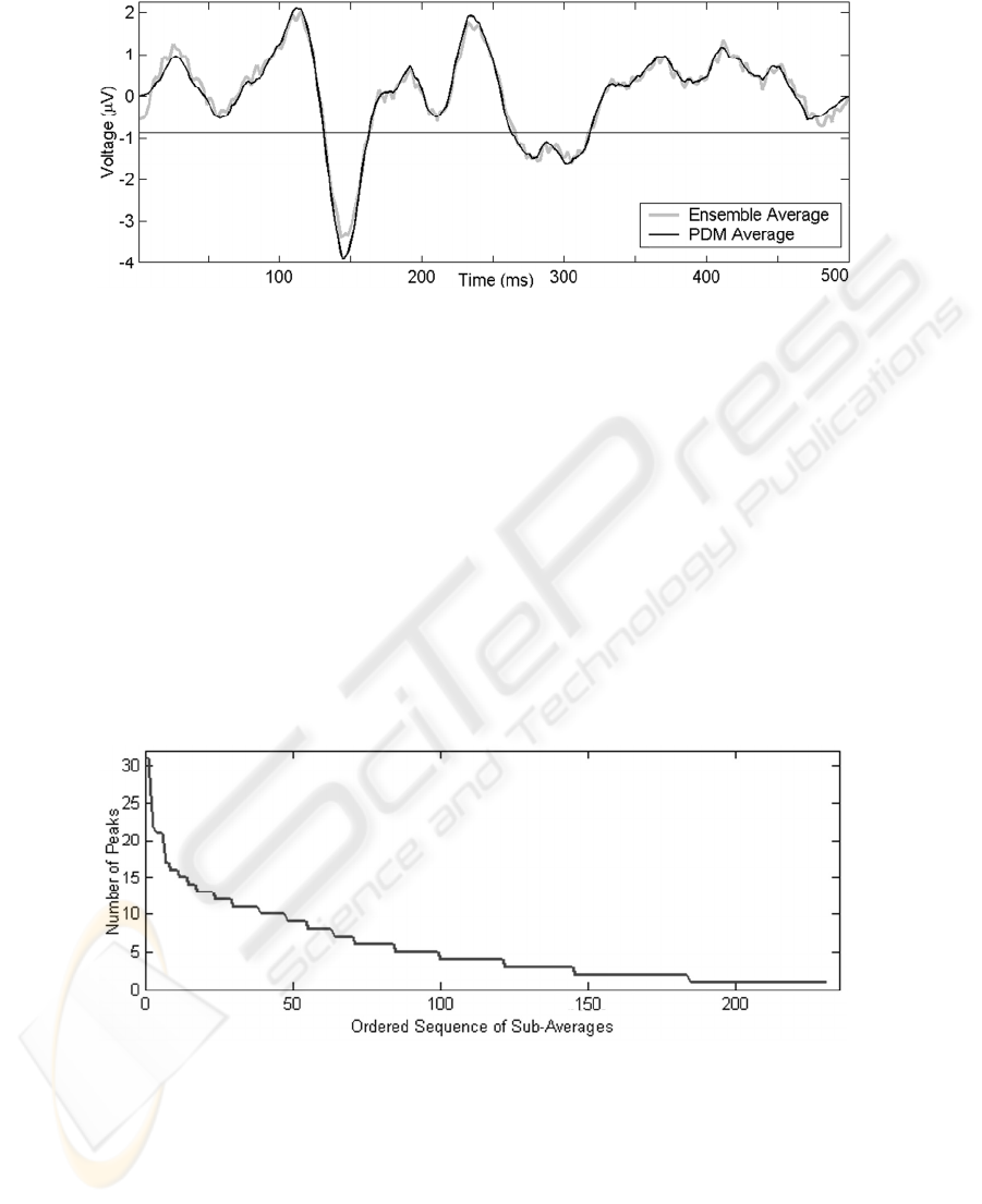
Fig. 1. Comparison of ensemble VEP average and sum of peak detected with PDM divided by
total number of peaks
The concentration matrices were generated from all the peaks across the 101
epochs used. From these matrices the location of the highest value in either matrix
was identified. Reading the matrix parameters for this location identifies that the
highest repetition was of a negative peak located at a latency of 144.5ms, with a
height of 8µV and a width of 31.25ms. Of the 101 epochs, 31 contain a peak with
similar characteristics to this. All peaks associated with this location were then
removed from the concentration matrix and the next highest value in either matrix
was identified. This process was iterated until both matrices were empty and all
peaks were grouped. The number of peaks in each group is charted in Fig. 2. In a
purely random system, one would expect a more horizontal trend however the left
hand skewness indicates identification of areas of increased concentration of EEG
activity. The summation of all 231 sub-averages yields the same PDM average
illustrated in Fig. 1.
Fig. 2. Histogram showing the ordered sequence of sub-average peaks versus number of peaks
within each sub-average.
8
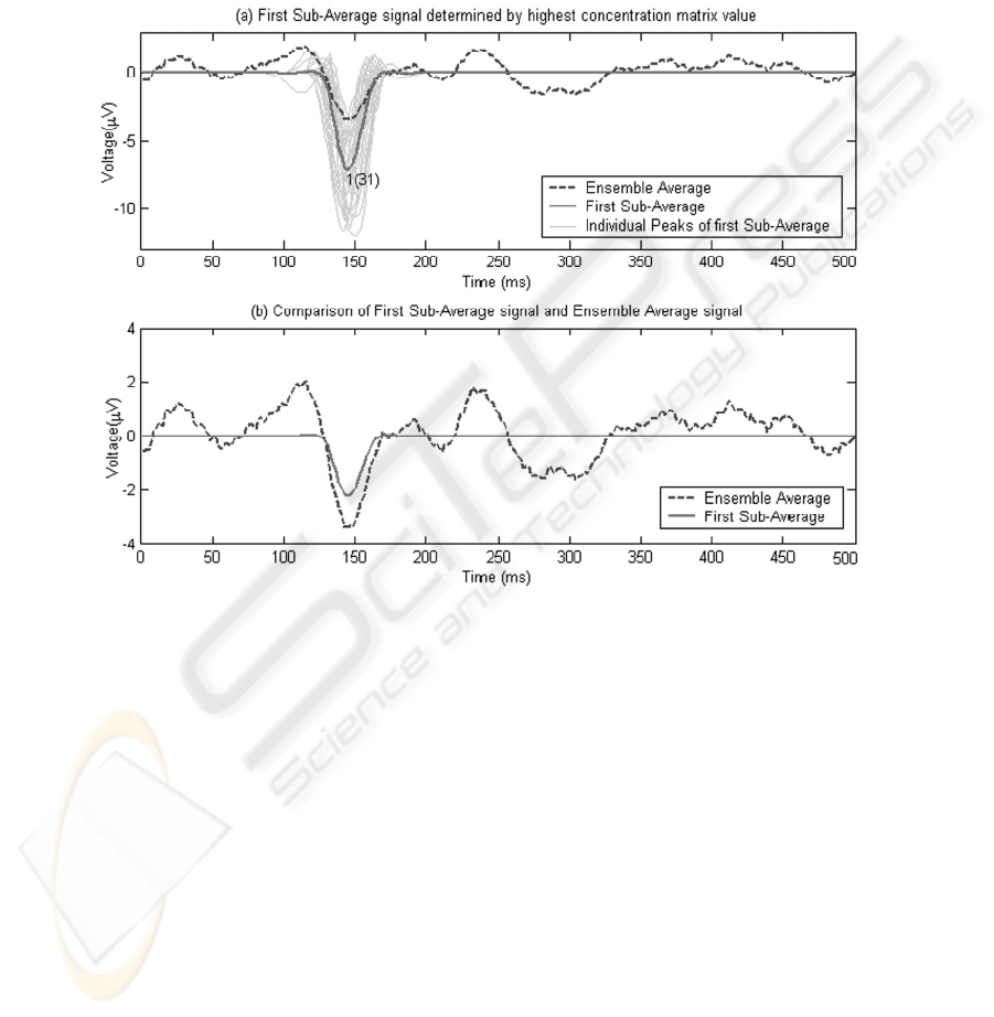
Results for the first sub-average are presented in Fig. 3. The ensemble average is
shown as a dashed line in both Fig. 3(a) and Fig. 3(b) for comparative purposes. In
Fig. 3(a), all 31 individual peaks of the first sub-average are plotted together with the
average of these 31 peaks. This is the actual average determined by summing all 31
peaks and dividing by the actual number of epochs selected, which is 31. Fig. 3(b)
illustrates the average of the 31 peaks determined by adding up all 31 peaks but
dividing by the total number of epochs which is 101 in this case.
Fig. 1. Examination of the First Sub-Average determined by the highest value in either
concentration matrix representing the similar peaks that occurs most often. In this case, there
are 31 peaks out of a possible 101 epochs.
The first sub-average in Fig. 3(b) is directly comparable with the Ensemble
Average since these are both averaged over the 101 epochs. It is a scaled version of
first sub-average in Fig. 3(a). This comparison gives a good indication of how the first
sub-average peak compares to the ensemble average peak in local area.
After calculating the first sub-average, the subsequent sub-averages were
calculated. The number of peaks identified in each sub-average group is charted in
Figure 2. It is observed that some sub-averages are more significant than others.
Based on this, a summation of the first 15 sub-averages is presented in Fig. 4. Again,
the ensemble average is shown as a dashed line in both Fig. 4(a) and Fig. 4(b) for
comparative purposes. The cumulative sub-average average by 31 epochs is shown in
9
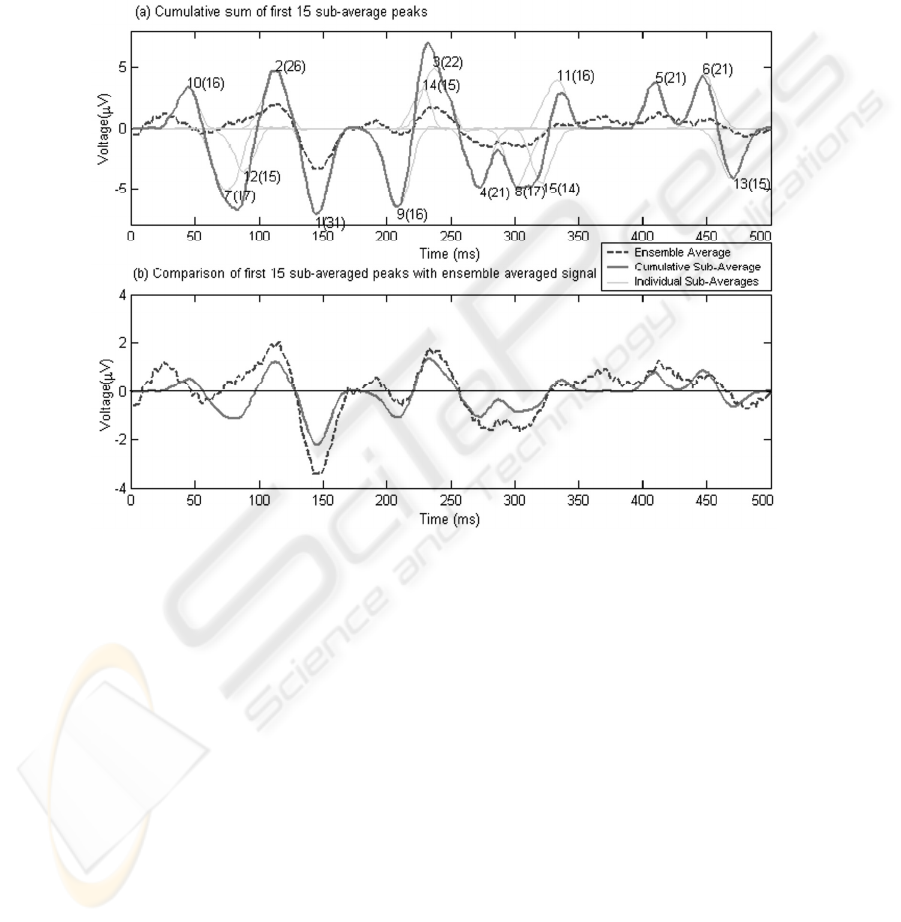
Fig. 4(a) and scaled by 101 epochs in Fig. 4(b) is shown by the thick straight line.
Individual sub-averages also shown in Fig. 4(a) as a light thin line.
It is noted from Fig. 4(b) that for the most part, the fifteen chosen sub-averages
correlate with major peaks of the ensemble average. These have been identified with
a lower number of epochs ranging from 31 down to 14. However, it is important to
note that the full 101 epochs needed to be calculated in order to pick out the sub-
averages.
Fig. 2. Examination of the first 15 Sub-Average signals. Indices in (a) are annotated as x(y)
where x is the order number for the sequence of sub-averages (1-15) and y is the number of
peaks in that sub-average (when x=1, y=31).
5 Discussion
It is observed that the summation of the 15 sub-averages in Fig. 4(b) retains the major
features of the ensemble average. These 15 sub-averages represent a total of just 283
peaks used out of a total of 1278 peaks originally identified in the 100 epochs of data.
Hence only 22% of the total Evoked Potential raw data is used to generate this
averaged evoked potential. It is also observed that this cumulative sub-average tracks
the standard ensemble average well. The notable exception is the appearance of a
negative peak at 82ms, which is not apparent in the ensemble average signal. Further
10

scrutiny of the remaining sub-averages reveals that in the ensemble average, this
peaks is cancelled out by a positive peak at this time position which has a large
magnitude but a small number of repetitions. This represents a possible advantage of
this system over the typical ensemble average system where such a peak is not
evident and could result in loss of information.
Separating overlapping peaks is an important and difficult component of any
singularity detection technique [6]. On occasion, some detected peaks do not have a
close fit to the original. However, it is observed that the vast majority of epochs give
an excellent fit to the original signal.
A new method of peak detection for evoked potentials has been presented. Using
an example of VEP based EEG data generated using 104 experiments, this peak
detection method is shown to retain the same evoked potential information as the
ensemble averaging technique. It is envisaged that this tool could help interpret the
visual evoked potential in two ways. Firstly, the higher concentration locations
indicate a more repeatable evoked potential signal and hence give a reliability factor
to the peak that is being viewed. Secondly, when cancellation of positive and
negative peaks occurs, the make-up of that cancellation may be examined in terms of
size of peak and number of times it occurs. Further testing and analysis of this
technique is being undertaken to broaden its application and to verify the results more
generally.
References
1. Grossman, A., Morlet, J.: Decomposition of Hardy Functions into Square Integrable
Wavelets of Constant Shape. SIAM J. Math. 15 (1984) 723-736
2. Demiralp, T., Yordanova, J., Kolev, V., Ademoglu, A., Devrim, M., Samar, V. J.: Time-
Frequency Analysis of Single-Sweep Event-Related Potentials by Means of Fast Wavelet
Transform. Brain and Language 66(1) (1999) 129-145
3. Maclennan, A. R., Lovely, D. F.: Reduction of Evoked Potential Measurement by a
TMS320 Based Adaptive Matched-Filter. Medeical Engineering & Physics 17(4) (1995)
248-256.
4. Quiroga, R. Q., van Luijtelaar, E. L. J M.: Habituation and Sensitization in Rat Auditory
Evoked Potentials: a Single-Trial Analysis with Wavelet Denoising. Int. Jour. Of
Psychophysiology 43 (2001) 141-153
5. Mallat, S., Hwang W. L.: Singularity Detection and Processing with Wavelets. IEEE
Transactions on Information Theory 38(22) (1992) 617-643
6. Melkonian, D., Blumenthal, T. D., Meares, R.: High Resolution Fragmentary
Decomposition – a Model Based Method of Non-Stationary Electrophysiological Signal
Analysis. Journal of Neuroscience Methods 131 (2003) 149-159
7. Mallet, S.: A Theory for Multiresolution Signal Decomposition: the Wavelet
Representation. IEEE Trans. on Pattern Analysis and Machine Intelligence 11(7) (1989)
674-693
8. Misulis, K. E.: Spehlmann’s Evoked Potential Primer, 2nd edn, Butterworth-Heinemann
(1994)
11
