Evolutionary Techniques for Neural Network

Optimization

Eva Volná

University of Ostrava, 30ht dubna st. 22, 701 03 Ostrava, Czech Republic

Abstract. The idea of evolving artificial networks by evolutionary algorithms is

based on a powerful metaphor: the evolution of the human brain. The

application of evolutionary algorithms to neural network optimization is an

active field of study. The success and speed of training of neural network is

based on the initial parameter settings, such as architecture, initial weights,

learning rates, and others. A lot of research is being done on how to find the

optimal network architecture and parameter settings given the problem it has to

learn. One possible solution is use of evolutionary algorithms to neural network

optimization systems. We can distinguish two separate issues for it: on the one

hand weight training, and on the other hand architecture optimization. Next, we

will focus on the architecture optimization and especially on the comparison of

different strategies of neural network architecture encoding for the purchase of

the evolutionary algorithm.

1 Genetic background for network topology optimization

The typical network considered here is a directed acyclic graph of simple neurons or

units. Each unit has a state, represented by a real number, a set of input connections,

and a set of output connections to other units. The connections themselves have real-

valued weights, w

. A unit’s state, o

is computed as a nonlinear function of the

weighted sum of the states of units from which it receives inputs. The nonlinear

activation function is a sigmoid, effectively endowing the unit with a threshold action;

the position of the threshold is controlled with a bias or „threshold weight“, q

. This is

summarized in equations:

)1(

−

∑

ijiji

ows

(1)

A subset of the units is designated as input units. These units have no input

connections from other units; their states are fixed by the problem. Another subset of

units is designated as output units; the states of these units are considered the result of

the computation. Units that are neither input nor output are known as hidden units.

Volná E. (2005).

Evolutionary Techniques for Neural Network Optimization.

In Proceedings of the 1st International Workshop on Artiﬁcial Neural Networks and Intelligent Information Processing, pages 3-11

DOI: 10.5220/0001191800030011

 SciTePress

A problem will specify a training set of associated pairs of vectors for the input units

and output units.

The full specification of a network to solve a given problem involves enumerating

all units, the connections between them, and setting the weights on those connections.

The first two tasks are commonly solved in an ad hoc or heuristic manner, while the

final task is usually accomplished with the aid of a learning algorithm, such as

backpropagation. Backpropagation [3], [5] is a supervised learning technique that

performs gradient descent on a quadratic error measure to modify connection weights.

A network begins with small random weights on its connections and is trained by

comparing its response to each stimulus in the training set with the correct one and

altering weights accordingly. The learning algorithm introduces new design variables,

such as the parameters to control rate of descent.

Genetic

Algorithm

ulation

Network

Performace

Evaluation

Sampling &Synthesis

of Network

„

Blue

rints“

blueprint fitness

estimates

instalation

ew, Untrained Network

testing

Trained Network

Training

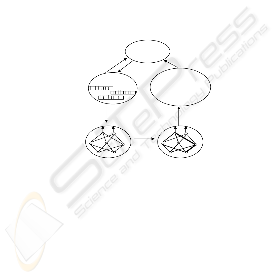
Fig. 1. A population of „blueprints“ designs for different neural networks - is cyclically

updated by the genetic algorithm based on their fitness scores. Fitness is estimated by

instantiating each blueprint into an actual neural network, training, and then testing the network

on the given task.

We use the genetic algorithm [2], [4] to search a space of possible neural network

architectures. In most of these experiences, the system begins with a population of

randomly generated networks. The structure of each network is described by a

chromosome or genetic blueprint - a collection of genes that determine the anatomical

proprieties of the network structure and the parameter values of the learning

algorithm. We use backpropagation to train each of these networks to solve the

problem and then evaluate the fitness of each network in a population. We define

fitness to be a combined measure of worth on the problem, which may take into

account learning speed, accuracy, and cost factors such as the size and complexity of

the network. Network blueprints from a given generation beget offspring according to

a reproductive plan that takes into consideration the relative fitness of individuals. In

this respect, application of the genetic algorithm is little different from any other

function optimalization application. A network spawned in this fashion will tend to

contain some attributes from both of its parents. A new network may also be a mutant,

differing in a few randomly selected genes from a parent. Novel features may arise in

either case: through synergy between the attributes of parents or through serendipitous

mutation. The basic cycle is illustrated in Figure 1 [2]. This process of training

individual networks, measuring their fitness, and applying genetic operators to

produce a new population of networks is repeated over many generations. If all goes

well, each generation will tend to contain more of the features that were found useful

in the previous generation.

2 Encoding strategies for neural network topology

We address two major shortcomings of this heuristic approach here. First, the space

of possible artificial neural network architectures is extremely large and most of

applications are unexplored. Second, what constitutes a good architecture is

dependent on the application. Both the problem that is to be solved and the constraints

on the neural network solution need to be considered, but at present we have no

techniques or methods for doing so. Optimal architecture is necessary achieved by

amount of manual trial-and-error experimentation. The problem of optimising neural

network structure for a given set of performance criteria is a complicated one. There

are many variables, both discrete and continuous, and they interact in a complex

manner. The evaluation of a given design is a noisy affair, since the efficacy of

training depends on starting conditions that are typically random. In short, the

problem is a local application for the genetic algorithm that is used to synthesise

appropriate network structures and values for learning parameters. Thumb rules like:

“the harder the problem the more units you need“ are of little practical use to the

design problem. It is known that a neural network with at least one hidden layer can

approximate every function. Almost always a fully interconnected architecture is

used. But what is the optimal number of units and their organization into layers? With

the exception of some simple task (e.g. the XOR-problem) humans cannot foresee the

optimal network topology.

Such complex spaces cannot be explored efficiently be enumerative, random or

even heuristic knowledge-guided search methods. In contrast, the adaptive features of

genetic algorithms (building blocks, step-width control by crossover) provide a more

robust and faster search procedure. Additionally, it is easy to speed-up the genetic

search by means of parallel processing.

Before we discuss the differences between several approaches we want to give a

basic genetic algorithm for topology optimization, which is common to all these

approaches. It is assumed that two representations of the networks are distinguished:

A) genotypes, which are modified by the genetic algorithm′s operators (e.g. mutation

and crossover); B) phenotypes, which are trained by a conventional learning

procedure (e.g. backpropagation) used for performance evaluation or selection.

Roughly two basic representation schemes can be distinguished: low-level genotypes

and high-level genotypes. While the first one is transparent and easy to use, there are

two variants of second representation scheme.

Low-level genotypes. Low-level genotypes directly code the network topology. Each

unit and each connection is specified separately. In [6] the following classification of

the encoding strategies of a neural network topology is proposed (the classes are

roughly ordered to the complexity of the strategies), e.g. direct encoding strategies:

− Connection-based encoding. The genome is a string of weight values or pure

connectivity information. The requires a fixed maximal architecture, which is

typically either fully-connected or layered [7]:

− Node-based encoding. The genome is a string or tree of node information. The

code for each node may include relative position, backward connectivity, weight

values, threshold function and more. An advantage over previous approach is that

more flexibility can be obtained by using nodes as basic units. The literature [8]

describe the genetic programming paradigm, which genetically breeds populations

of computer programs to solve problems, where the individuals in the population

are hierarchical compositions of functions and arguments of various sizes and

shapes (i.e. LISP symbolic expressions: S - expression).

− Layer-based encoding. With layer-based encoding we can obtain larger networks

[9]. The encoding scheme is a complicated system of descriptions of connectivity

between a list of layers.

− Pathway-based encoding. Pathway-based encoding is proposed in [10], [11] for

recurrent neural network. The network is viewed as a set of paths from an input to

an output node.

High-level genotypes. High-level genotypes are more complex coded representations

of network architectures. They can be further divided into parametric and recipe

genotypes. There are the networks splited into modules of units which are specified

by parameters and which are coupled by parametric connectivity patterns, in

parametric genotypes. Even through this representation is more compact and thus well

suited to code large network architectures, it is difficult to choose the relevant

parametric shapes.

− The graph generation grammar (GGG) developed by [13] is an early grammar

encoding method based on context-free and deterministic Lindenmayer systems,

e.g. L-systems [12]. The grammar contains productions rules in the special form.

− Nolfi and Parisi in [14] described a method for encoding neural network

architecture into a genetic string, which is inspired by the characteristics of neural

development in real animals. The neurons are encoded with coordinates in a two-

dimensional space. The mapping from genes to neurons is direct in a sense, but the

connections are grooving in a special manner.

− In [15] are proposed main theoretical advantages of the use of L – systems to code

network topologies over “blueprint representations” where the evolutionary

algorithm specifies every single connection in neural networks. They used a

version of L - systems to grow the networks (e.g. the context-sensitive L - system

to rewrite neurons and modules of neurons). Here is each neuron/module by

default connected to the next adjacent neuron/module, and missing connections are

denoted by comma.

− Channon and Damper in [16] investigated evolving of behaviors of artificial life

creatures with natural selection. They decided to evolve neural networks and they

used L-systems for encoding of the topology. Precisely, a context-free L - system

was designed for the evolution of neural networks. Specific attention was paid to

producing a system in which children’s networks resemble aspects of their parents.

− In [17] is proposed a method based on L-system that directs neural mass growth

inspired in biology. Rules are then applied in 2-dimensional cell matrix, instead of

a string.

− Gruau´s [18] cellular encoding method uses a grammar tree to encode a cellular

developmental process to grow neural networks. The decoding starts from a

network with a single hidden “cell” that is connected all input and output neurons

of the network. The cell starts reading the grammar tree from its root. The nodes of

the tree are instructions that control how the cell is divided, etc. The child cells of a

differentiate by moving their “read-heads” to different branch of the grammar tree.

Over the last decade many systems have been developed that evolve no only a neural

network topology but both the topology and the parametric values of a neural network

[19], [20] etc.

3 Theoretical basis

We can choose any combination of the n hidden neurons to flip their weight signs so

there are (see Formula 2) structurally different but functionally identical networks

generated by this transformation.

⎛

⎝

⎜

⎞

⎠

⎟

∑

(2)

Suppose that we have a network with h

... h

as hidden nodes. The mapping

implemented by the network does not change if a particular hidden node with all its

incoming and outgoing weights is exchanged with another neuron and its weights. For

instance the networks h

... h

and h

... h

are equivalent, even though the first

and second neuron have changed their position in the hidden layer. Obviously we can

permute any of the n neurons so the total number of functional equivalent networks

by this transformation is n!.

Since the two transformations are independent of each other, there is a total of

n! functional equivalent but structurally different networks. Recently it has also

been proven that at least in the case of a single hidden layer, one output neuron and a

tangent hyperbolic transfer function the weights within this group of symmetries is

unique, so there are exactly 2

n! redundant networks for a specific mapping.

Suppose a we would tell that h hidden units and l hidden layers are necessary for a

given problem. Now, we have to distribute the hidden units into these layers. We will

derive a recursive formula which allows to compute the number of possible partitions

p(h,l). It is evident that:

1. If l = 1 or if h = l then p(h,l) = 1.

2. If h < l then p(h,l) = 0, because empty partitions are not reasonable.

3. If h > l we get p(h,l) = p(h - 1, l -1) + p(h - 1, l).

By this formula we can compute the number of possible partitions from that number

of a less complex architecture with h - 1 units. The first term counts the number of

partitions if the boundary of an additional layer separates the additional unit itself.

The second term means that the additional unit is placed into the last hidden layer of a

less complex architecture which has already l layers.

If we have decided for a specific partition we are confronted with the problem of

optimizing connectivity. For h hidden units the number of possible connections is

limited by two extreme topologies which are fully interconnected from input layer

(m units) to output layer (n units):

− A topology that has as much as possible hidden layers with one hidden unit each.

We will refer to that topology as TALL.

− A topology that has just one hidden layer. It forms a look-up table and we will

refer to it as WIDE.

While the TALL-architecture contains (see Formula 3) connections, the WIDE-

architecture has only (see Formula 4) connections, but in most practical applications

neither the TALL - nor the WIDE - architecture will be best suited. Thus, have to find

a connectivity pattern, which is adapted to a particular task.

()

hmn mn

−

+⋅ + + ⋅

(3)

(

)

Chmnm

=⋅ + +⋅n

(4)

4 Conclusion

Genetic algorithms are an effective optimisation, search and machine learning

technique, suitable for a large class of problems, especially for NP-complete state

space problems, which cannot easily be reduced to close form. Genetic algorithms

have been applied largely to the problem of training a neural net, as an alternate

technique to more traditional methods like backpropagation.

Neural network adaptation. Neural networks solve XOR problem that is not linearly

separable and in this case we cannot use neural network without hidden units. Each

network architecture is 2 - 2 - 1 (e.g. two units in the input layer, two units in the

hidden layer, and one unit in the output layer). The nets are fully connected. If is the

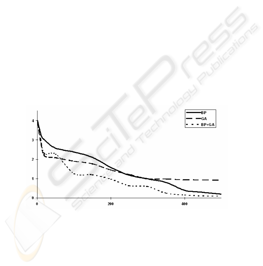
XOR problem solved with genetic algorithm (GA), we need the following parameters:

number of generation was 500, probability of mutation is 0.01 and probability of

crossover is 0.5. The initial population contains 30 neural networks with randomly

generated weight values. Every weight value is written in a code as well as in [21].

Genetic operators (mutation and crossover) also are defined in [21]. History of the

average error function of the whole population during calculation is shown in the

Figure 2. Global search such as genetic algorithms are usually computationally

expensive to run. If the XOR problem is solved with the method backpropagation

(BP), we need the following parameters: learning rate is 0.4 and momentum is 0.1.

History of its error function during whole calculation is shown in the Figure 2. There

is shown an average value of the error function, because the adaptation with

backpropagation algorithm was applied 30 during 500 cycles. If the XOR problem is

solved with a method that combines genetic algorithm and backpropagation, then all

parameters and genetic operators are the same as stated above. And besides that we

have to define the following parameters: number of backpropagation´s iterations is 10

and probability of backpropagation is 0.2. If the input condition of backpropagation is

fulfilled (e.g. if a randomly number is generated, that is equal to the defined constant),

all individuals are then adapted with 10 cycles of BP. History of the average error

function of the whole population during calculation is shown in the Figure 2.

iteratio

Error

Fig. 2. History error function during calculation, where BP is adaptation with backpropagation,

GA is adaptation with genetic algorithm, BP+GA is adaptation with method that combines

genetic algorithm and backpropagation.

This paper also introduces theoretical proposes of neural network configuration by

using genetic algorithms [1], [7], [8], [9] etc. In this participation has been done

simple initial study on neural network optimization by means of evolutionary

techniques and given positive results has shoved that evolutionary techniques can be

used in this way. In the future more complex study on neural network optimization

are going to be done by means of another evolutionary algorithms.

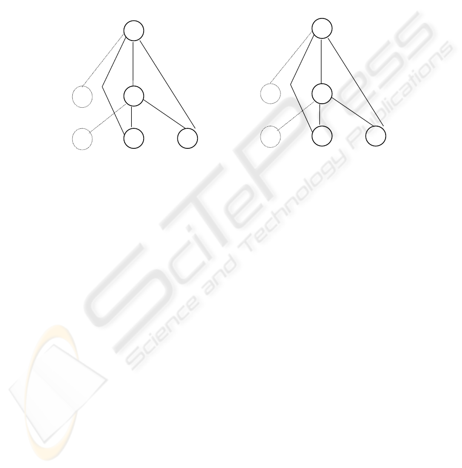
Neural network architecture. Neural networks solve XOR problem. The Figure 3

illustrates the best representation of neural network for the solution of XOR problem

(a) that was found with genetic algorithm [21] and its following adaptation with

backpropagation (b).

-6.6

10.3

-6.2

-12.7

-7.2

-8.8

-2.2

-7.2

11.2

-7.1

-15.5

-7.5

-7.9

-3.5

bias

(a)

(b)

Fig. 3. The best representation of neural network for solution of XOR problem with genetic

algorithm (a) and its following adaptation with backpropagation (b).

References

1. Arena, P. - Caponetto, R. - Fortuna, L. - Xibilia, M.G.: M.L.P. optimal topology via genetic

algorithms. Proceedings of the international conference in Innsbruck, pp. 671-674, Austria

1993.

2. Beale, R. - Jackson, T.: Neural Computing: An Introduction. J W Arrowsmith Ltd, Bristol,

Greit Britain 1992.

3. Goldberg, D. E.: Genetic algorithm in search optimalization and machine learning.

Addison-Wesley, Reading., Massachusets 1989.

4. Herz, J. - Krogh, A. - Palmer, R. G.: Introduction to the Theory of Neural Computation.

Addison Wesley Publishing Company, Redwood City 1991.

5. Lawrence, D.: Handbook of genetic algorithms. Van Nostrand Reinhold, New York 1991.

6. Köhn, P. Genetic encoding strategies for neural networks. Master’s thesis, University of

Tennessee, Knoxville, IPMU, 1996.

7. Maniezzo, V. Searching among search spaces: Hastening the genetic evolution of

feedforward neural networks. In R. F. Albrecht, C. R. Reeves, and N. C. Steele, editors:

Artificial Neural Nets and Genetic Algorithms. Springer-Verlag, pp. 635-643 (1993).

8. Koza, J. R. and J. P. Rice. Genetic generation of both the weights and architecture for a

neural network. In Proceedings of the International Joint Conference on Neural Networks,

Volume II, IEEE Press, 1991.

9. Harp, S. A., Samad, T., and Guha, A. Towards the genetic synthesis of neural networks. In

J. D. Schaffer, Ed. San Mateo eds.: Proc. of the Third Intl. Conf. on on Genetic Algorithms

and Their Applications. CA: Morgan Kaufmann pp. 360—369, (1989).

10. Jacob, C., Rehder, J. Evolution of neural net architectures by a hierarchical grammar-based

genetic system. In Proceedings of the International Joint Conference on Neural Networks

and Genetic Algorithms, Innsbruck, pp. 72-79. (1993

11. Angeline, P. J., G. M. Saunders, and J. B. Pollack. An evolutionary algorithm that constructs

recurrent neural networks. IEEE Transactions on Neural Networks, 5: 54-65, 1993.

12. Lindenmayer A.: Mathematical models for cellular interaction in development I, II. Journal

of Theoretical biology (18): 280-315 1968.

13. Kitano, H. Design neural network using genetic algorithm with graph generation system.

Complex systems,(4): 461-476, 1990.

14. Nolfi, S., Parisi, D. Genotypes for neural networks. In M. A. Arbib, editor: The Handbook

of Brain Theory and Neural Networks. MIT Press 1995.

15. Boers, E.J.W., Kuiper, H., Happel, B.L.M., and Sprinkhuizen-Kuyper, I.G.. Designing

modular artificial neural networks. In H.A. Wijshoff, editor: Proceedings of Computing

Science in The Netherlands. pp. 87-96, Amsterdam, 1993. SION, Stichting Mathematisch

Centrum. Amsterdam 1993.

16. Channon, A. D. and Damper, R. I. Evolving novel behaviors via natural selection, In Adami,

C., Belew, R. K., Kitano, H. and Taylor, C. E., eds.: Alife IV. Sixth International

Conference on Artificial life. , pp. 384-388. Bradford Books/MIT Press, Cambridge, MA,

1998.

17. Aho, I., Kemppainen, H., Koskimies, K., Mäkinen, E., and Niemi, T. Searching neural

network structures with L systems and genetic algorithms. International Journal of

Computer Mathematics, 73 (1): 55-75, 1999.

18. Gruau, F., D. Whitley, and L. Pyeatt. A comparison between cellular encoding and direct

encoding for genetic neural networks. In J. R. Koza, D. E. Goldberg, D. B. Fogel, and R. L.

Riolo, editors, Genetic Programming 1996: Proceedings of the First Annual Conference, pp.

81-89, Cambridge, MA, MIT Press, 1996.

19. Opitz, D. W. and J. W. Shavlik. Connectionist theory refinement: Genetically searching the

space of network topologies. Journal of Artificial Intelligence Research, 6: 177-209, 1997.

20. Yao, X. and Y. Liu. Towards designing artificial neural networks by evolution. Applied

Mathematics and Computation, 91(1): 83-90, 1996.

21. Volna, E.. Learning algorithm which learns both architectures and weights of feedforward

neural networks. Neural Network World. Int. Journal on Neural & Mass-Parallel Comp. and

Inf. Systems. 8 (6): 653-664, 1998.