On Cluster Analysis Via Neuron Proximity in Monitored

Self-Organizing Maps

Susana Vegas-Azc

arate and Jorge Muruz

abal

Statistics and Decision Sciences Group

University Rey Juan Carlos, 28933 M

ostoles, Spain

Abstract. A potential application of self-organizing or topographic maps is clus-

tering and visualization of high-dimensional data. It is well-known that an ap-

propriate choice of the degree of smoothness in topographic maps is crucial for

obtaining sensible results. Indeed, experimental evidence suggests that suitably

monitored topographic maps should be preferred as they lead to more accurate

performance. This paper reconsiders the basic toolkit for cluster analysis —based

on the relative distance from each pointer to its immediate neighbours on the

network— from this monitoring perspective. It is shown that the idea works

nicely, that is, much useful information can be encoded and recovered via the

trained map alone (ignoring any possible density estimate available). Moreover,

the fact that a topographic map is not restricted to metric vector spaces makes

this learning structure a perfect tool to deal with biological data, such as DNA

or protein sequences of living organisms, for which only a similarity measure is

readily available.

1 Introduction

We are living the blast of the silicon-based biology era, an era in which investigation

of complete genomes is viable for the ﬁrst time. We need computer-based technologies

to cope with the vast quantities of data generated by genome projects, seeking not only

increased facilities in data storage and access, but also assistance in computational ma-

nipulation and post-processing. Without methods that help us to analyze this deluge of

data, the information it contains becomes useless.

The Self-Organizing Map (SOM) [1] is a popular neural network model for unsu-

pervised learning that tries to ‘imitate’ the self-organization process taking place in the

sensory cortex of the human brain (by which neighboring neurons will typically be ac-

tivated by similar stimuli). This model develops a mapping from a d-dimensional input

space, into an equal or lower-dimensional discrete lattice with regular, ﬁxed topology.

Thanks to a simple competitive learning process — whereby only weights connected to

the winner (or best matching unit) and its neighbours are updated—, the SOM structure

is often organized (topologically ordered).

We are interested in applying the SOM neural structure for sound clustering of

biological signals. We have a particular application in mind, namely, clustering pro-

teins. This problem has some tradition in the literature [2, 3], and it prompts a number

of interesting issues, beginning with the issue of the ‘vectorial vs. nonvectorial’ data

Vegas-Azcárate S. and Muruzábal J. (2005).

On Cluster Analysis Via Neuron Proximity in Monitored Self-Organizing Maps.

In Proceedings of the 1st International Workshop on Biosignal Processing and Classiﬁcation, pages 50-59

DOI: 10.5220/0001192800500059

 SciTePress

representation. However, in this paper we consider only the vectorial case and pursue

some foundational research (i) focusing on the use of interneuron proximity information

alone, and (ii) emphasizing the need to monitor the training process. While both theory

and applications have developed substantially in the SOM literature, there is probably

not a wide awareness yet (among practitioners) of the technical requirements for the

extracted maps, nor there seems to be a wide consensus on how to best monitor, train

or even analyze the SOM structure.

For clustering purposes, a good density estimate of the sampling distribution can

of course be very valuable, and certain kernel-based learning algorithms are naturally

suited to yield such estimates. While conventional kernel-based estimates [4, 5] seem

to provide generally good results, drawbacks in higher dimensions should still occur in

the multivariate case [6]. Recent approaches to SOM training usually incorporate some

statistical machinery yielding richer models and more principled ﬁtting algorithms (the

standard framework lacks a statistical model for the data and thus provides no density

estimate).

As regards monitoring, we have introduced an early-stopping criterion called UDL

(for uniform data load) and we have shown that it provides sensible density estimates

in a wide array of cases [7]. Here we show that the UDL criterion is also useful for

the usual basic proximity summaries (available in all training algorithms). To this end,

four algorithms are tested. Speciﬁcally, the batch version (SOM-B) [1] and a convex

adjustment (SOM-Cx) [8] of the standard SOM algorithm are compared to two kernel-

based learning rules: the generative topographic mapping (GTM) [9] and the kernel-

based maximum entropy learning rule (kMER) [10]. The latter three tend to achieve the

‘equiprobabilistic state’ that motivates the UDL criterion [7]; it appears unlikely that

SOM-B can achieve this state, but it is still monitored in the same way for the sake of

reference.

The organization is as follows. Section 2 brieﬂy describes the four topographic map

formation algorithms considered in the paper. Section 3 spells out the particular training

and testing strategies examined in the experiments reported in section 4. Some conclu-

sions are drawn in section 5.

2 SOM training algorithms

Before we actually describe the details of the algorithms, it is appropriate to begin with

a bit of background for the work presented here. As often noted, the quality of the SOM

ﬁt will be assessed in the ﬁrst place by the extent to which the organization or topology

preservation property holds. A substantial amount of research has been devoted to the

formalization and quantiﬁcation of this idea. Proposed approaches vary from the early

measures based entirely on the map pointers [11] to increasingly sophisticated variants

that also incorporate some aspects of the data into the analysis [12–15]. While much

progress has been done in the area, there is no universally accepted methodology for

practitioners to follow. Many proposed measures are not easy to interpret, and the avail-

able implementations are scarce. At any rate, empirical conﬁrmation is needed in each

case.

Determination of the most sensible criterion is also complicated by the nature of the

training algorithms. Most importantly, algorithms differ in their magniﬁcation factors,

that is, in the ability to reﬂect exactly the true density generating the data. When the

match between pointer density and data density is exact (at least asymptotically) we

talk of equiprobabilistic maps [16]. These have been argued to overcome the output

unit underutilization problem found in the standard SOM training algorithm. But even

among theoretically equiprobabilistic algorithms there are, as we shall see, substantial

differences in practical behaviour.

Finally, training algorithms vary also in the amount of modelling machinery in-

volved. As noted above, the traditional SOM structure lacks a statistical model for the

data, whereas modern training algorithms like GTM and kMER provide an explicit den-

sity estimate that can be very useful for clustering purposes. These estimates enhance

the framework and raise questions about the preferred training strategy.

Denote the SOM weight or pointer vectors as w

∈ IR

, i = 1, ..., N, and the data

as v

∈ IR

, m = 1, ..., M . In this paper we consider 2D SOMs only; besides, we

restrict consideration to squared maps equipped with the standard topology.

2.1 SOM-batch (SOM-B)

The batch version of Kohonen’s SOM training algorithm (SOM-B) is deﬁned by the

recursive update [1]

m=1

∗

m=1

∗

where H is the neighborhood function, typically chosen with a Gaussian shape and a

monotonically decreasing range, and i

∗

= arg min

{kv

− w

k} is the best matching

unit for the input data vector v

. Since SOM-B contains no learning rate parameter, no

convergence problems arise, and more stable asymptotic values for the weights w

’s are

obtained [1].

2.2 Convex adjustment (SOM-Cx)

A convex adjustment for the original SOM algorithm has been studied by Zheng and

Greenleaf [8]. They actually present two nonlinear models of weight adjustments. One

of them uses a convex transformation to adjust weights. This is seen to provide more

efﬁcient data representation for vector quantization, whereas the convergence rate is

comparable to that of the linear model. Speciﬁcally, the standard competitive learning

rule

∆w

= ηH

∗

− w

becomes

∆w

= ηH

∗

− w

)

where κ is a positive odd integer [8] and η represents the learning rate (which can also

be a monotonically decreasing function of time [1]).

2.3 Generative Topographic Mapping (GTM)

GTM [9] deﬁnes a non-linear mapping y(x, W ) from an L-dimensional latent space to a

d-dimensional data space, where L < d (and typically equals 2). By suitably constrain-

ing the model to a lattice in latent space, a posterior distribution over the latent grid

is readily obtained using Bayes’ theorem for each data point. More speciﬁcally, GTM

training is based on a standard EM procedure aimed at the standard Gaussian-mixture

log-likelihood [9]

log ℓ =

m=1

log

(

i=1

p(v

|i)P (x

)

, (1)

where P (x

) is the prior mass at each point in the latent grid and p(·|i) is the Gaussian

density centered at y

= y(x

, W ) (equal, of course, to our more common w

) and

spherical covariance with common variance σ

= β

−1

. A generalized linear regression

model is typically chosen for the embedding map, namely y(x, W ) = W Φ(x), where

Φ = Φ(x) is a matrix containing the scores by B ﬁxed basis functions and W is a free

matrix to be optimized together with β.

Note that the (optimized) quantity in Eq. 1 provides a standard measure on which a

GTM model can be compared to other generative models. Note also that the topology-

preserving nature of the GTM mapping is an automatic consequence of the choice of

a continuous function y(x, W ) [9]. Basis functions parameters explicitly govern the

smoothness of the ﬁtted manifold.

2.4 Kernel-based Maximum Entropy learning Rule (kMER)

kMER [10] was introduced as an unsupervised competitive learning rule for non-para-

metric density estimation, whose main purpose is to obtain equiprobabilistic topo-

graphic maps on regular, ﬁxed-topology lattices. Here, the receptive ﬁelds of neurons

are (overlapping) radially symmetric kernels, whose radii are adapted to the local input

density together with the weight vectors that deﬁne the kernel centroids. A neuron w

‘activated’ by an input data v

if it is contained within the hypersphere S

centered at

and with radius σ

. Since hyperspheres are allowed to overlap, several neurons can

be active for a given input vector. An online together with a batch version of kMER are

developed in [10]. We focus here on the online version of kMER, that is,

∆w

= η

j=1

(v)Sgn(v

− w

where Sgn(·) is the sign function taken componentwise, Ξ is a fuzzy code membership

function and H is the time-decreasing neighborhood function. Note that, unlike GTM,

kMER derives a different standard deviation σ

for each mixture Gaussian component.

Speciﬁcally, the kernel radii σ

are adjusted so as to verify, at convergence, that the

probability of each neuron i to be active is given by a ﬁxed scale factor ρ (which controls

the degree of overlap between receptive ﬁelds).

It can be seen that the receptive ﬁeld weight centers and its radii are adapted to

achieve a topographic map maximizing the unconditional information-theoretic entropy

[16]. Furthermore, the density estimate output by kMER can be written in terms of a

mixture distribution where the kernel functions represent the component Gaussian den-

sities with equal prior probabilities, providing an heteroscedastic, homogeneous mix-

ture density model [16] whose log-likelihood function can be computed just like in the

GTM case (see Eq. 1 above).

3 Analysis

Once we have trained the SOM, a number of summaries of its structure are routinely

extracted and analyzed. In particular, here we consider Sammon’s projections, median

interneuron distances, and dataloads. We now review each of this basic tools in turn.

To visualize high-dimensional SOM structures, use of Sammon’s projection is cus-

tomary. Sammon’s map provides a useful global image while estimating all pairwise

Euclidean distances among SOM pointers and projecting them directly onto 2D space.

Thus, since pointer concentrations in data space will tend to be maintained in the pro-

jected image, we can proceed to identify high-density regions directly on the projected

SOM. Furthermore, by displaying the set of projections together with the connections

between immediate neighbours, the degree of self-organization in the underlying SOM

structure can be assessed intuitively in terms of the amount of overcrossing connections.

Interneuron distance or proximity information has also been traditionally used for

cluster detection in the SOM literature. Inspection of pointer interdistances was pio-

neered by Ultsch, who deﬁned the uniﬁed-matrix (U-matrix) to visualize Euclidean dis-

tances between neuron weights in Kohonen’s SOM. Here we consider the similar me-

dian interneuron distance (MID) matrix. Each MID entry is the median of the Euclidean

distances between the corresponding pointer and all pointers belonging to a star-shaped,

ﬁxed-radius neighborhood containing typically eight units. The median can be seen as a

conservative choice; more radical options based on extremes can also be implemented.

To facilitate the visualization of pointer concentrations, a linear transformation onto a

256-tone gray scale is standard (the interpretation here is that the lower the value, the

darker the cell).

On the other hand, the number of data vectors projecting onto (won by) each unit,

namely the neuron dataload, is the main quantity of interest for UDL monitoring pur-

poses. Again, to easily visualize the dataload distribution over the map, a similar gray

image is computed, namely, the DL-matrix (note that, in this case, darker means higher).

The main idea in UDL is that, in the truly equiprobabilistic case, each neuron would

cover about the same proportion of data, that is, a (nearly) uniform DL-matrix should

be obtained. Hence, training is stopped as soon as the ﬁrst signs of having reached this

state are noticed [7]. Note that we use the UDL stopping policy as a heuristic for the

optimal value of the ﬁnal adaptation radius in SOM-B and SOM-Cx.

The training strategy for cluster analysis is thus formally described as follows. First

train the SOM network until a (nearly) uniform DL-matrix is obtained and Sammom’s

projection shows a good level of organization. Compute the MID and DL matrices

associated to this map. We stress that we do not use the maps obtained by training all

the way (which yield much worse results).

Now, a cluster detection strategy based on MID would ﬁrst isolate all local maxima

on the MID surface and identify each such a mode with a speciﬁc cluster in the data.

We can also consider a minimum Euclidean labelling scheme, in which each neuron is

marked with the label that occurs most within its activation region. We denote this as

the labels matrix below.

4 Experimental work

We now summarize our main experimental results. We ﬁrst analyze a trimodal 2D data

set with two of the modes close enough to illustrate the ﬁner detail in our algorithms.

Next we examine a mixture of gaussians with clusters relatively apart from each other.

Finally, we consider a real data set with ten clusters in high-dimensional input space.

4.1 Three modes in 2D space (3M-2D)

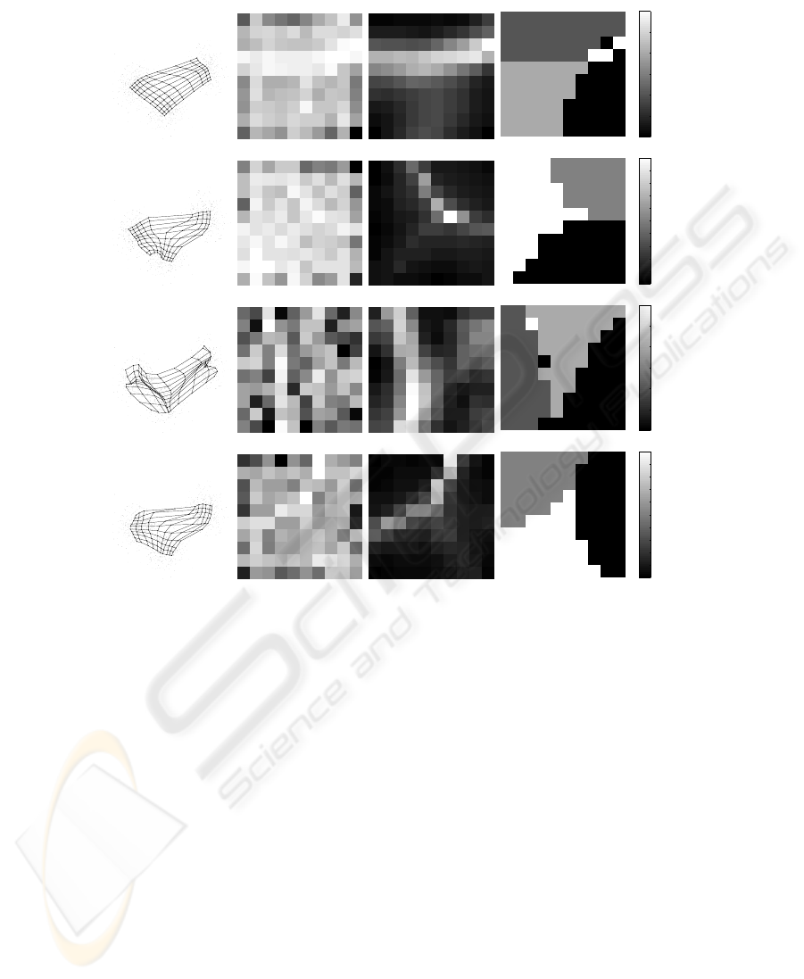
Figure 1 shows good organization and suitable DL matrices in all cases (albeit more

uniform DL matrices can be seen in the case of GTM and kMER). As a result, the three

clusters are correctly identiﬁed via MID analysis, yet we note that kMER and SOM-Cx

provide the cleanest assignments.

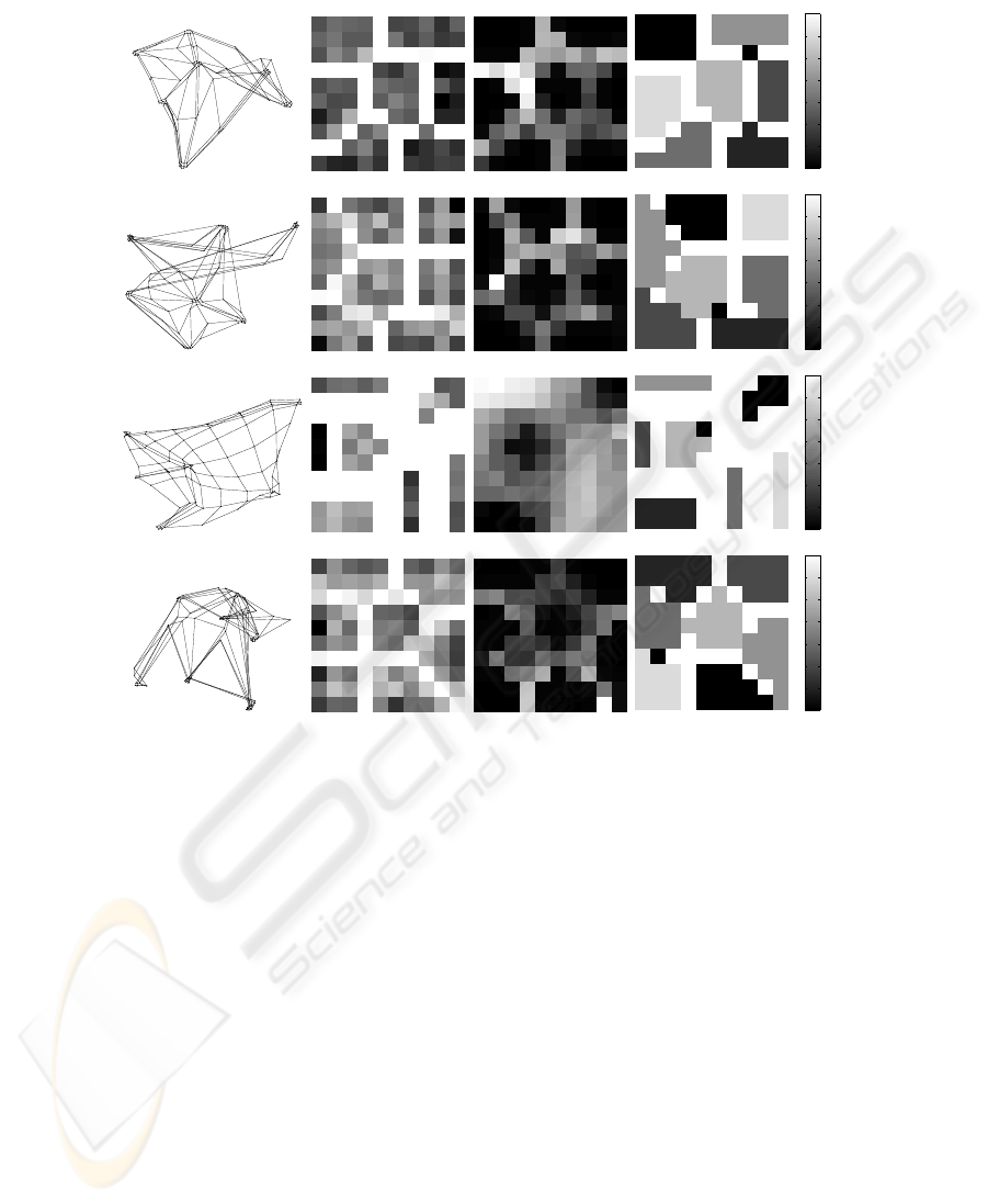
4.2 Seven modes in 5D space (7M-5D)

Data are generated in a two-step process. We ﬁrst sample the locations of the cluster

centroids, then sample each cluster in term. All Gaussians are spherical, and all clus-

ters have the same size. The standard deviation of the centroid distribution is much

larger than that of the data (clusters are well separated). Figure 2 shows generally nice

behaviour except in the GTM case, where a relatively high number of dead units is un-

expectedly observed. In all other cases, the seven clusters are exhibited very clearly by

the MID matrices.

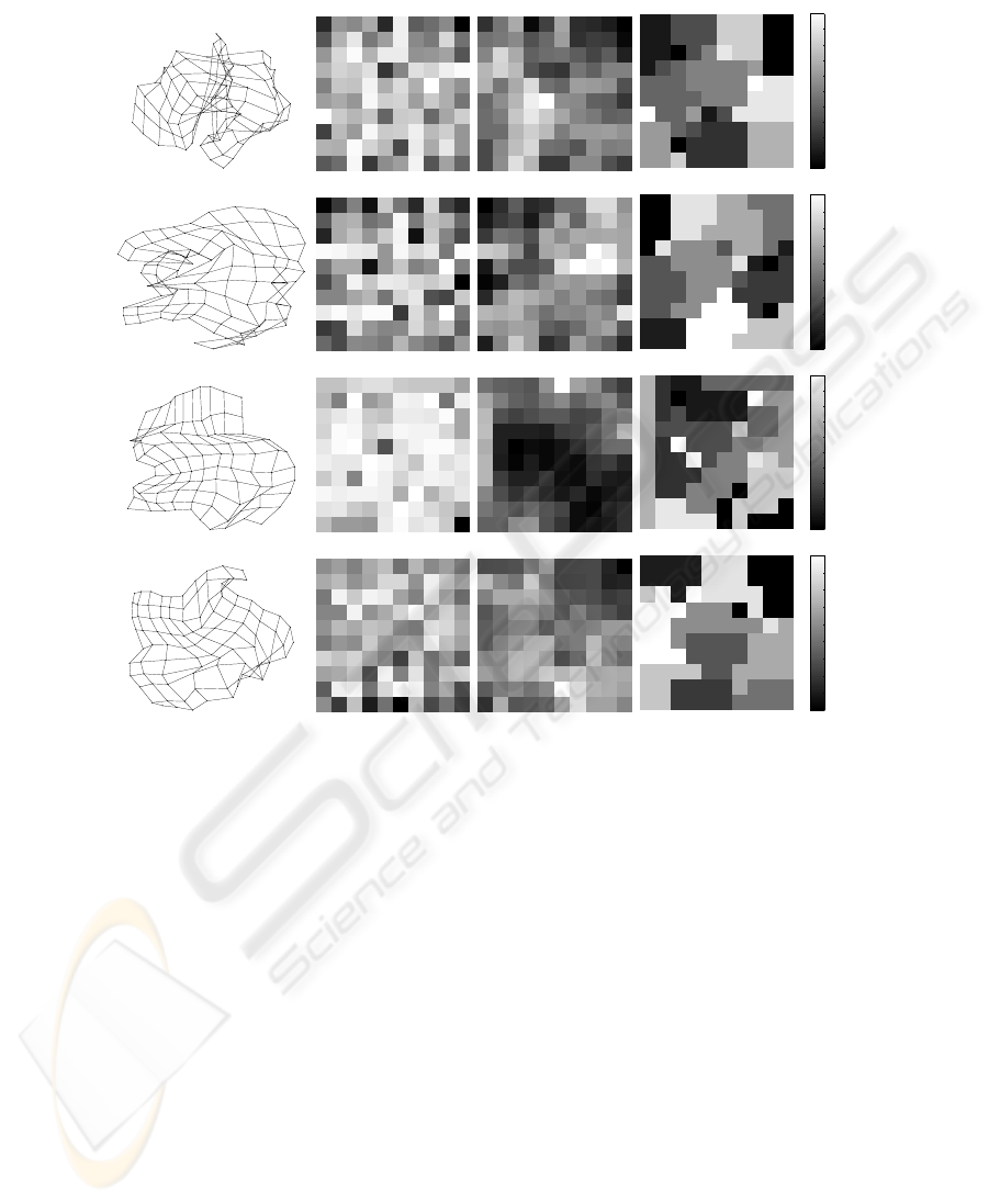
4.3 Real-world example

We now take up the Multiple Features database from the well-known UCI repository,

which we call the Mfeat data. Here d = 649 and there are M = 2, 000 training vectors

available. As Figure 3 shows, interestingly organized maps obtain in all cases. These

maps involve rather uniform DL matrices and result in pretty good cluster recognition,

see also [7]. Here we see GTM ranking worst in terms of cluster separation.

5 Summary and conclusions

We have revisited a universal approach to cluster detection based on the SOM structure

and neuron proximity. We have shown that good results are obtained most of the time

when maps are monitored (stopped early) via the UDL criterion introduced in [7]. Early

stopping seems indeed almost a requirement if the ultimate goal of the analysis depends

Sammon−3M2D−CarrSu−som−batch−sd

DL−3M2D−CarrSu−som−batch−sd

MID−3M2D−CarrSu−som−batch−sd

1.5

2.5

3.5

Labels−3M2D−CarrSu−som−batch−sd

Sammon−3M2D−CarrSu−som−cx−sd

DL−3M2D−CarrSu−som−cx−sd

MID−3M2D−CarrSu−som−cx−sd

1.2

1.4

1.6

1.8

2.2

2.4

2.6

2.8

Labels−3M2D−CarrSu−som−cx−sd

Sammon−3M2D−CarrSu−gtm−udl

DL−3M2D−CarrSu−gtm−udl

MID−3M2D−CarrSu−gtm−udl

1.5

2.5

3.5

Labels−3M2D−CarrSu−gtm−udl

Sammon−3M2D−CarrSu−kmer−sd

DL−3M2D−CarrSu−kmer−sd

MID−3M2D−CarrSu−kmer−sd

1.2

1.4

1.6

1.8

2.2

2.4

2.6

2.8

Labels−3M2D−CarrSu−kmer−sd

a b c d

Fig.1. Performance by SOM-B (top), SOM-Cx (middle-up), GTM (middle-down) and kMER

(bottom) on 3M-2D data set: (a) trained maps with data set highlighted; (b) DL matrices; (c)

MID matrices; (d) Labels matrices

on having a faithful approximation to the data-generating distribution. Other stopping

criteria can be seen in [13].

Perhaps the Gaussian kernels in GTM are too constrained by the transformation

from lattice to input space, for it appears that these kernels cannot move freely when

needed at some point along the training process. We have also seen that many of the

previous drawbacks are avoided by kMER, which produces more ﬂexible and more

effective maps, yet SOM-B and SOM-Cx seem also very well behaved and quite useful

in the cases studied.

The scope of the above ideas for SOM-based biosignal clustering is important in as

much as vectorial data keep on being worked out by researchers. Our results should be

reassuring for practitioners following strategies based on neuron proximities, but they

should also be recalled of the need to monitor map formation closely.

sammon−7M5D−som−batch−sd

DL−7M5D−som−batch−sd

MID−7M5D−som−batch−sd

Labels−7M5D−som−batch−sd

sammon−7M5D−som−cx−sd

DL−7M5D−som−cx−sd

MID−7M5D−som−cx−sd

Labels−7M5D−som−cx−sd

Sammon−7M5D−gtm−udl

DL−7M5D−gtm−udl

MID−7M5D−gtm−udl

Labels−7M5D−gtm−udl

sammon−7M5D−kmer−sd

DL−7M5D−kmer−sd

MID−7M5D−kmer−sd

Labels−7M5D−kmer−sd

a b c d

Fig.2. Performance by SOM-B (top), SOM-Cx (middle-up), GTM (middle-down) and kMER

(bottom) on 7M-5D data set: (a) Sammon projected maps; (b) DL matrices; (c) MID matrices;

(d) Labels matrices

Sammon−mfeat−som−batch−sd

DL−mfeat−som−batch−sd

MID−mfeat−som−batch−sd

Labels−mfeat−som−batch−sd

Sammon−mfeat−som−sd

DL−mfeat−som−sd

MID−mfeat−som−sd

Labels−mfeat−som−sd

Sammon−mfeat−gtm−udl

DL−mfeat−gtm−udl

MID−mfeat−gtm−udl

Labels−mfeat−gtm−udl

Sammon−mfeat−kmer−sd

DL−mfeat−kmer−sd

MID−mfeat−kmer−sd

Labels−mfeat−kmer−sd

a b c d

Fig.3. Performance by SOM-B (top), SOM-Cx (middle-up), GTM (middle-down) and kMER

(bottom) on Mfeat data set: (a) Sammon projected maps; (b) DL matrices; (c) MID matrices; (d)

Labels matrices

References

1. Kohonen, T.: Self-Organizing Maps. Springer-Verlag, 3rd extended ed., Berlin (2001)

2. Ferr

an, E.A., Ferrara, P.: Topological maps of protein sequences. Biological Cybernetics 65

(1991) 451–458

3. Kohonen, T., Somervuo, P.: How to make large self-organizing maps for nonvectorial data.

Neural Networks 15 (2002) 945–952

4. Gray, A.G., Moore, A.W.: Nonparametric density estimation: Toward computational

tractability. In Barbar

a, D., Kamath, C., eds.: SDM: Proceedings of the Third SIAM In-

ternational Conference on Data Mining, San Francisco, CA, USA, May 1-3, 2003, SIAM

(2003)

5. Davies, P.L., Kovac, A.: Densities, spectral densities and modality. Annals of Statistics 32

(2004) 1093–1136

6. Scott, D.W., Szewczyk, W.F.: The stochastic mode tree and clustering. Journal of Computa-

tional and Graphical Statistics (2000)

7. Muruz

abal, J., Vegas-Azc

arate, S.: On equiprobabilistic maps and plausible density estima-

tion. In: 5th Workshop On Self-Organizing Maps, Paris. (2005)

8. Zheng, Y., Greenleaf, J.F.: The effect of concave and convex weight adjustements on self-

organizing maps. In: IEEE Transactions on Neural Networks. Volume 7-1. (1996) 87–96

9. Bishop, C.M., Svens

en, M., Williams, C.K.I.: Gtm: The generative topographic mapping.

Neural Computation 10 (1997) 215–235

10. Van Hulle, M.M.: Kernel-based equiprobabilistic topographic map formation. Neural Com-

putation 10(7) (1998) 1847–1871

11. Bauer, H.U., Pawelzik, K.: Quantifying the neighborhood preservation of self-organizing

feature maps. IEEE Trans. Neural Networks 3 (1992) 570–579

12. Kaski, S., Lagus, K.: Comparing self-organizing maps. In von der Malsburg, C.,

v.S.W.V.J.C., Sendhoff, B., eds.: Proceedings of ICANN’96, International Conference on

Artiﬁcial Neural Networks, Lecture Notes in Computer Science. Volume 1112., Springer,

Berlin (1996) 809–814

13. Villmann, T., Der, R., Herrmann, M., Martinetz, T.: Topology preservation in self-organizing

feature maps: Exact deﬁnition and measurement. IEEE Trans. Neural Networks 8(2) (1997)

256–266

14. Lampinen, J., Kostiainen, T.: Overtraining and model selection with the self-organizing map.

In: Proc. IJCNN’99, Washington, DC, USA. (1999)

15. Haese, K., Goodhill, G.J.: Auto-som: Recursive parameter estimation for guidance of self-

organizing feature maps. Neural Computation 13 (2001) 595–619

16. Van Hulle, M.M.: Faithful representations and topographic maps: From distortion- to

information-based self-organization. Wiley, New York (2000)