
A RECURRENT NEURAL NETWORK RECOGNISER FOR ONLINE
RECOGNITION OF HANDWRITTEN SYMBOLS
Bing Quan Huang and Tahar Kechadi
Department of Computer Science, University College Dublin,
Belfield, Dublin 4, Ireland
Keywords:
Recurrent neural network, gradient descent method, learning algorithms, Markov chain model, fuzzy logic,
feature extraction, context layers.
Abstract:
This paper presents an innovative hybrid approach for online recognition of handwritten symbols. This ap-
proach is composed of two main techniques. The first technique, based on fuzzy logic, deals with feature
extraction from a handwritten stroke and the second technique, a recurrent neural network, uses the features
as an input to recognise the symbol. In this paper we mainly focuss our study on the second technique. We
proposed a new recurrent neural network architecture associated with an efficient learning algorithm. We
describe the network and explain the relationship between the network and the Markov chains. Finally, we
implemented the approach and tested it using benchmark datasets extracted from the Unipen database.
1 INTRODUCTION
A recogniser model is very important for any pat-
tern classification system. For handwriting recogni-
tion, most recogniser systems have been built based
on rule based methods or statistical methods, such
as motor model (Plamondon and Maarse, 1989;
Schomaker and Tteulings, 1990), primitive decompo-
sition (S. Bercu, 1993), elastic matching (C.C.Tappet,
1984), time-delay neural network (M. Schnekel and
Henderson, 1994; Seni and Nasrabadi, 1994), and
hidden Markov models (J.Hu and W.Turin, 1996;
S. Bercu, 1993). However, these systems analyse ab-
stract descriptions of handwriting to identify symbols
or words. The problem with these methods is that it
is in most cases impossible to design an exhaustive
set of rules that model all possible ways of forming a
letter (Subrahmonia and Zimmerman, 2000).
Generally, the performance of a recognizer that em-
ploys statistical methods is more flexible and reliable.
The common static methods – curve/feature matching
(C.C.Tappet, 1984), Markov Model based approach
and Neural Network based approaches, have their
own disadvantages. The difficulty of the curve/feature
matching approach is that they are computationally
intensive and impractical for large vocabulary of
handwriting (C.C.Tappet, 1984) (e.g. elastic match-
ing (M. Schnekel and Henderson, 1994; C.C.Tappet,
1984)). Hidden Markov Models (HMMs) (Rabiner,
1989) have been successfully applied firstly to speech
recognition (L.R. Bahl and Mercer, 1983; S.E. Levin-
son and Sondhi, 1983) and have recently been used
to solve sequence learning problems, including online
handwriting recognition (J.Hu and W.Turin, 1996;
T.Wakahara and K.Odaka, 1997). However, HMMs
suffer from a weak discriminative power and requires
a human expert to choose a number of states with ini-
tial estimates of the model parameters and transition
probability between the states (Rabiner, 1989). Time
delay neural network (TDNN) (M. Schnekel and Hen-
derson, 1994; Seni and Nasrabadi, 1994) trained
with Back-propagation algorithm (R.J.Williams and
Zipser, 1995) require the setting of less parameters.
However, the limitation of TDNN is that the input
fixed time window can cause it to be unable to deal
with varying the length of sequences.
Based on another type of dynamic neural networks,
called recurrent neural networks, which successfully
deals with temporal sequences such as formal lan-
guage learning problems (Elman, 1999), it overcomes
the problem of TDNN and it is easy to use as a recog-
nizer. The two common types of recurrent networks
are the Elman network and fully recurrent networks
(Williams and Zipser, 1989) (RTRL). However, El-
man networks face difficulties due to their architec-
ture: the network’s memory consists of one context
27
Quan Huang B. and Kechadi T. (2005).
A RECURRENT NEURAL NETWORK RECOGNISER FOR ONLINE RECOGNITION OF HANDWRITTEN SYMBOLS.
In Proceedings of the Seventh International Conference on Enterprise Information Systems, pages 27-34
DOI: 10.5220/0002514200270034
Copyright
c
SciTePress

layer (relatively small), the direct connection of hid-
den layer to the output layer, and the computation
cost, which heavily depends on the size of the hid-
den layer. The main difficulty with the fully recurrent
network with real time recurrent learning is its com-
putational complexity.
Therefore, a new recurrent network architecture
with a new dynamic learning algorithm is proposed.
It is shown that this network is computationally more
efficient than RTRL. In addition, the overhead of
its dynamic learning algorithm is much smaller than
the overhead of RTRL computations. We use semi-
discrete features which are extracted by using fuzzy
logic techniques to reduce the technique overhead and
to improve its accuracy
The recognition process begins with feature extrac-
tion. For each handwritten symbol, a set of features
is generated whereby each feature is one of three
types: Line, C-shape or O-shape. We believe that
the most intuitive way to describe any symbol is as
a combination of these basic feature types. Fuzzy
logic (L.A.Zadeh, 1972) is used to extract the fea-
tures, which is more appropriate given the amount
of imprecision and ambiguity present in handwritten
symbols and also to reduce the amount of data to be
processed during the recognition phase. The feature
extraction result is encoded and used as the input to
the network. The isolated digit data base of UNIPEN
(Guyon and Janet, 1994) Train-R01/V07 is used to
train and test the network.
The paper is organised as follows. Section 2 gives
an overview of the feature extraction phase. In sec-
tion 3 the network architecture is presented. Section
4 describes the network learning algorithm. Section
5 shows experimental results and section 6 contains
conclusions and prospects for future work.
2 FEATURE EXTRACTION
Feature extraction is a process, which transforms the
input data into a set of features, which characterise the
input, and which can therefore be used to classify the
input. This process has been widely used in attempts
at automatic handwriting recognition (O. D. Trier and
Taxt, 1996). Due to the nature of handwriting with
its high degree of variability and imprecision, obtain-
ing these features is a difficult task. A feature ex-
traction algorithm must be robust enough that for a
variety of instances of the same symbol, similar fea-
ture sets should be generated. Here we present a fea-
ture extraction process in which fuzzy logic is used
(J.A.Fitzgerald and T.Kechadi, 2004). Fuzzy logic is
particularly useful for extracting features from hand-
written symbols (Gomes and Ling, 2001) (Malaviya
and Peters, 1997), because a greater understanding
Figure 1: Example of a feature Extraction Process applied
on a digit 5
of what is present in the symbol is achieved and ul-
timately a more informed decision can be made re-
garding the identity of each symbol.
Chording Phase: Each handwritten symbol is rep-
resented by a set of strokes {s
0
, . . . , s
v
}, where each
stroke is a sequence of points. This raw input data
is rendered more suitable for feature extraction by
a pre-processing phase called chording. Chording
transforms each stroke s into a chord vector
−→
C =
hc
0
, . . . , c
n−1
i, where each chord c
i
is a section of s
which approximates a sector of a circle. This phase
simplifies the input data so that feature extraction
rules can be written in terms of chords rather than se-
quences of points. Furthermore, chording identifies
the locations in the stroke where new features may
begin, so the number of sections of the stroke which
need to be assessed as potential features is reduced.
Feature Extraction Phase: The chord vectors
h
−→
C
0
, . . . ,
−→
C
v
i are the input to the feature extraction
phase, in which the objective is to identify the fea-
ture set for the symbol. The feature set will be the
set of substrokes F = {̟
0
, . . . , ̟
m−1
} encompass-
ing the entire symbol which is of a higher quality than
any other possible set of substrokes. Each substroke
̟
j
is a sequence of consecutive chords {c
a
, . . . , c
b
}
from a chord vector
−→
C
i
= (c
0
, . . . , c
n−1
), where
0 ≤ a ≤ b ≤ n and 0 ≤ i ≤ v.
The quality of a set of substrokes, represented by
ζ(F ), is dictated by the membership of the substrokes
in F corresponding to feature types. We distinguish
three types of feature: Line, C-shape and O-shape.
The membership of a substroke ̟
j
in the set Line,
for example, is expressed as µ
Line
(̟
j
) or Line(̟
j
),
and represents the confidence that varpi
j
is a line. In
the definition of ζ(F ) below, Γ is whichever of the
fuzzy sets Line, C-shape or O-shape ̟
j
has highest
membership in.
ζ(F ) =
m−1
j=0
µ
Γ
(̟
j
)
m
(1)
Fuzzy Rules: The membership of a fuzzy set is
determined by fuzzy rules. The fuzzy rules in the
rule base can be divided into high-level and low-level
ICEIS 2005 - ARTIFICIAL INTELLIGENCE AND DECISION SUPPORT SYSTEMS
28
rules. The membership of a fuzzy set correspond-
ing to feature types is determined by high-level rules.
Each high-level fuzzy rule defines the properties re-
quired for a particular feature type, and is of the
form:
Γ(Z) ← P
1
(Z) ∩ . . . ∩ P
k
(Z) (2)
This means that the likelihood of a substroke Z be-
ing of feature type Γ is determined by the extent to
which the properties P
1
to P
k
are present in Z. The
membership of a fuzzy set corresponding to proper-
ties is determined by low-level fuzzy rules. In each
low-level rule the fuzzy value P
i
(Z) is defined in
terms of values representing various aspects of Z. To
express varying degrees of these aspects we use fuzzy
membership functions such as the S-function (Zadeh,
1975).
The strength of our feature extraction technique
is therefore dependent on an appropriate choice of
requisite properties for each feature type, and low-
level fuzzy rules which accurately assess the extent
to which these properties are present. These proper-
ties and rules were continually updated and improved
over time until the memberships being produced for
the feature types were deemed accurate.
Algorithm: The fuzzy rules form the basis of a fea-
ture extraction algorithm, which determines the best
feature set using numerous efficiency measures. For
example, initial detection of the sharp turning points
in the symbol can lead to a significant reduction in the
number of substrokes to be evaluated, on the basis that
such points usually represent boundaries between fea-
tures. Also, the investigation into a substroke being a
particular feature type halts as soon as an inappropri-
ate property is identified.
Example: For the symbol shown in Figure 1, the
effect of feature extraction is a partition of the in-
put
−→
C = {c
0
, . . . , c
4
} into a set of features F =
{(c
0
, c
1
), (c
2
), (c
3
, c
4
)}, where µ
Line
(c
0
, c
1
) = 0.66,
µ
Line
(c
2
) = 0.98, and µ
Cshape
(c
3
, c
4
) = 0.93.
Encoding the Feature Extraction Result: The
feature extraction result F must be encoded before
it can be used as input to the network. Each feature
̟ is represented by five attributes: type, orientation,
length, x-center and y-center, which are explained be-
low.
• Type: Whichever of the sets Line, C-shape or O-
shape ̟ has highest membership in. The numeric
value is 0 if ̟ is of type O-shape, 0.5 if its of type
Line and 1.0 if its of type C-shape.
• Orientation: If ̟ is of type Line, its orientation
is the direction in which it was drawn (between 0
◦
and 360
◦
). If ̟ is of type C-shape, its orientation
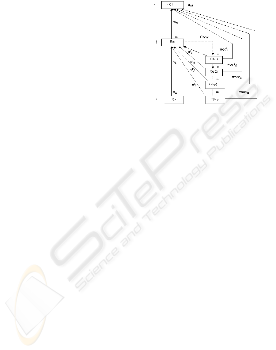
Figure 2: The network architecture
is the direction in which it is facing. Features of
type O-shape are assigned an orientation of 0
◦
.
• Length: The length of ̟ as a fraction of the sym-
bol length.
• X-centre: This value represents the horizontal po-
sition of ̟ within the symbol. The closer it is to
the right, the higher the value.
• Y-centre: This value represents the vertical posi-
tion of ̟ within the symbol.
3 THE RECURRENT NETWORK
A new recurrent neural network has been proposed by
(B.Q. Huang and Kechadi, 2004). It is based on the
Elman network type architecture (Elman, 1999). This
network is characterised by two key features. The net-
work is provided with a multi-context layer (MCL)
(Wilson, 1996), which plays a role of the network
memory. It allows the network to store more appli-
cation states. The second feature is the feed-forward
connectivity between the MCL and the output layer,
which can reduce the number of neurons in the hidden
layer (B.Q. Huang and Kechadi, 2004). The architec-
ture of this network is shown in Figure 2.
3.1 Basic notations and definitions
The following notations and definitions are used to
explain our network functionality.
• Net inputs and Outputs: Let n
in
, n
out
and m de-
note the number of input, output, and hidden layer
units respectively. Let n
con
be the number of active
context layers, and let the total number of context
A RECURRENT NEURAL NETWORK RECOGNISER FOR ONLINE RECOGNITION OF HANDWRITTEN
SYMBOLS
29
layers be denoted by q. The number of units in each
context layer is the same as in the hidden layer.
Let t be the current time step. I
i
(t) is the input
of neuron i in the input layer,
˜
h
j
(t) is the input
of neuron j in the hidden layer, and ˜o
k
(t) is the
input of neuron k in the output layer. The output
of the hidden and output layers are H(t) and O(t)
respectively. The output of neuron l of a context
layer p is denoted by C
l
(t − p), and d
k
(t) is the
target of neuron k in the output layer.
• Connection weights: Let v
ji
be the weight con-
nection from the input layer to the hidden layer and
u
p
kl
be the weight connection from the p
th
context
layer to the hidden layer. Let woc
p
kl
be the weight
connection from the p
th
context layer to the output
layer and w
kj
be the weight connection from the
hidden layer to the output layer.
The selection of the network activation function
according to the application (Lawrence et al., 2000)
is very important for a successful implementation of
the network. For the symbol recognition the softmax
function and logistic function are selected as the ac-
tivation functions for the output layer and the hidden
layer respectively, written below:
f
SM
(x
i
) =
e
x
i
N
i
′
=1
e
x
i
′
f(x
i
) =
1
1 + e
x
i
where x represents the i
th
net input, and N is the
total number of net inputs. The derivatives of the ac-
tivation functions can be written respectively as fol-
lows:
f
′
SM
(x
i
) = (1 − f
SM
(x
i
))f
SM
(x
i
)
f
′
(x
i
) = (1 − f (x
i
))f(x
i
)
According to the architecture of the network, the
output of the hidden layer and the output layer are
calculated at every time step, while the outputs of the
context layers are obtained by shifting the information
from p to p + 1 for (p = 1 to q). The first context
layer is updated by the hidden layer, as shown in Fig.
1. This is done in a feed-forward fashion:
1. The net input and output of the hidden layer units
are calculated respectively as follows:
˜
h
j
(t) =
n
in
i=1
I
i
(t)v
ji
(t)+
n
con
p=1
m
l=1
C
l
(t−p)u
p
jl
(t) (3)
H
j
(t) = f(
˜
h
j
(t)) (4)
where C
l
(t − p) are the outputs of the context
layers obtained by copying the output of its prede-
cessor. The context layer gets the previous output
of the hidden layer. The following equations sum-
marise this operation:
C
j
(t − p) = C
j
(t − p + 1), p = 2, ..., q (5)
C
j
(t − 1) = H
j
(t) (6)
2. The net input and output of the output layer are
given respectively as follows:
˜o
k
(t) =
m
j=1
H
j
(t)w
kj
(t) +
n
con
p=1
m
l=1
C
l
(t − p)woc
p
kl
(t)
(7)
O
k
(t) = f
SM
(˜o
k
(t)) (8)
3.2 The Network and Markov Chain
Any system based on our network architecture pre-
dicts the current state depending on the previous states
window [(t − 1) → (t − p)]. When p = 1,
the network expresses a Markov chain model that
predicts the current state based only on the pre-
vious one. However, the Markovian assumption
of conditional independence is one of the limita-
tions. The network tries to predict a more accu-
rate current state based on more historical states.
Thus, the network expresses an extended probabil-
ity model based on Markov chain. The main fo-
cus is on the recurrent part of the network because
it plays a magic role when the system deals with se-
quence modeling tasks (Lawrence et al., 2000). In
an m-states Markov model (MM) (Rabiner, 1989)
for which the transition matrix is A = {a
ij
} and
the distribution probability vector is Ξ([Obsq, t)) =
{ρ
1
(Obsq, t), ρ
2
(Obsq, t), · · · , ρ
n
(Obsq, t)]}, where
n is the length of the observation sequence Obsq, the
Markov chain equations can be written as
ρ
j
(Obsq, t + 1) =
m
i=1
a
ji
ρ
i
(Obsq, t), j = 1, · · · , m. (9)
Ξ(Obsq, t + 1) = AΞ(Obsq, t), (10)
where A ≥ 0,
P
m
j
a
ij
= 1. Let I(t) =
{I
1
(t), · · · , I
in
(t)}, H(t) = {H
1
(t), · · · , H
m
(t)},
C(t − p) = {C
1
(t −p), · · · , C
m
(t −p)}, and O(t) =
{O
1
(t), · · · , O
out
(t)}. We write the state-transition
and output functions, defined by (3), (4), (7), and (8),
as:
H(t) = f (I(t), C(t − 1), · · · , C(t − p))
= f (I(t), H(t − 1), · · · , H(t − p))
(11)
and
O (t) = f
SM
(H(t), C(t − 1), · · · , C(t − p))
= f
SM
(H(t), H(t − 1), · · · , H(t − p))
(12)
According to the formulaes (3), (4), (5), (6) and
(11), the state-transition map f can be written as a
set of maps parameterised by input sequence s as fol-
lows:
f
p
s
(x) = f(φ
1
(s), · · · , φ
p
(s), x) (13)
Given an input sequence S = {s
1
, s
2
, · · · , s
t
}, the
current state after t step is
H(t) = f
p
s
p
···s
t
(H(0)) = f
p
S
t
1
(H(0)) (14)
When p = 1, the above formulae (11), (12), (13),
and (14) are re-written respectively as follows:
H(t) = f(I(t), H(t − 1)) (15)
ICEIS 2005 - ARTIFICIAL INTELLIGENCE AND DECISION SUPPORT SYSTEMS
30
O (t) = f
SM
(H(t), H(t − 1)) (16)
f
1
s
(x) = f(φ
1
(s), x) = f(φ
1
(s), x) (17)
H(t) = f
1
s
1
···s
t
(H(0)) = f
S
t
1
(H(0)) (18)
For p = 1, the current state (at time t) of the sys-
tem depends only on the previous state (at time t − 1).
The equations (15), (17), and (18) express the prop-
erty of a Markov chain (see equations (9) and (10)).
However, when p > 1 the current state (at time t) de-
pends on more historical states, which are stored in
the previous states window [(t− 1) → (t −p)], which
is out of the Markovian assumptions of conditional
independence. Therefore, for p > 1, the system is ex-
pressed as a general probability or stochastic model,
within a given time window.
3.3 The Network Dynamics
The network is designed such that, given a set of fea-
tures it attempts to predict the associated symbol. It-
eratively, for each input symbol an ordered sequence
of features are fed to the network. For each feature,
the network generates ten outputs expressed as pre-
diction rates for all the associated symbols. Note that
if probabilities of each feature are used to track the
procedures of the digit prediction, and the maximum
output probability of the last feature is used to identify
the digit, then the network works in a similar fashion
to Markov chains to solve grammar problem. Firstly,
according to a given feature, the network estimates a
score for each digit (see Table 1). When the last fea-
ture was presented, the output symbol was identified
according to the highest score that results in firing its
corresponding neuron. The Table 1 shows an exam-
ple of how the symbol 5, with three features, is recog-
nised. The scores were given, in percentage, for each
symbol (or output neuron) expressing if the feature is
present. When the last feature was presented to the
network the highest score is returned by the neuron
number 5, recognising the digit 5.
Table 1: The output confidence levels of the tested symbol
The output probabilities with associated all digits (%)
0 1 2 3 4 5 6 7 8 9
0 4.2 10.9 34.4 0 5.3 0 44.9 0 0.3
0 7.7 4.4 3.1 0 73.8 0 10.3 0.1 0.7
0.4 25.8 1.4 1.7 0 67.3 0 0.4 3.0 0
4 THE NETWORK LEARNING
ALGORITHM
The common training algorithms usually used for re-
current network (RNN) are based on the gradient de-
scent method to minimise the error output. With
Back-propagation through the time (BPTT) (Wer-
bos, 1990; R.J.Williams and Zipser, 1995) one needs
to unfold a discrete-time RNN and then applies the
back-propagation algorithm. However, BPTT fails to
deal with long sequence tasks due to the large mem-
ory required to store all states of all iterations. The
RTRL learning algorithm established by (Williams
and Zipser, 1989) for a fully recurrent network com-
putes the derivatives of states and outputs with re-
spect to all weights at each iteration. It can deal
with sequences of arbitrary length, and requires less
memory storage proportional to sequence length than
BPTT. The recognition of handwritten symbols is a
lengthy task, therefore we update the learning algo-
rithm (B.Q. Huang and Kechadi, 2004) which is simi-
lar to RTRL, according to the gradient descent method
for this network.
The choice of a cost function for the cross-entropy
measure should be based on the type of classification
problem (Lawrence et al., 2000). When classifying
handwritten symbols the network output is a range of
confidence values, so this is a multinomial classifica-
tion problem. Therefore, the cross-entropy error for
the output layer is expressed by the following:
E(t) = −
n
out
k=1
d
k
(t) ln O
k
(t) (19)
The goal is to minimise the total network cross-
entropy error. This can be obtained by summing the
errors of all the past input patterns:
E
total
=
T
t=1
E(t) (20)
Up to this point we have introduced how the net-
work works and is evaluated. Now, we use the gradi-
ent descent algorithm to adjust the network parame-
ters, called the weight matrix W . Firstly, we compute
the derivatives of the cross-entropy error for each net
input of the output layer, the hidden layer, and the
context layer. These are called local gradients. The
equations for the output layer, hidden layer, and con-
text layer are written respectively as follows:
LG
k
(t) = d
k
(t) − O
k
(t) (21)
LG
j
(t) =
n
out
k=1
LG
k
(t)w
kj
(t) (22)
LG
p
l
(t) =
n
out
k=1
LG
k
(t)woc
p
kl
(t) (23)
The partial derivatives of the cross-entropy error
with regard to the weights between the hidden and
output layers (w
kj
(t)) and the weights between out-
put layer and multi-context layer (woc
p
kl
(t)) are as fol-
lows:
∂E(t)
∂w
kj
(t)
= LG
k
(t)H
j
(t) (24)
∂E(t)
∂woc
p
kl
(t)
= LG
k
(t)C
l
(t − p) (25)
A RECURRENT NEURAL NETWORK RECOGNISER FOR ONLINE RECOGNITION OF HANDWRITTEN
SYMBOLS
31
The derivation of the cross-entropy error with re-
gards to the weights between the hidden and multi-
context layer is
∂E(t)
∂u
p
jl
(t)
= −
m
j
′
=1
LG
j
′
(t)
∂H
j
′
(t)
∂u
p
jl
(t)
+
n
con
p
′
=1
m
r=1
LG
p
′
r
(t)δ
rj
′
∂H
j
′
(t − p
′
)
∂u
p
jl
(t)
(26)
where
∂H
j
′
(t)
∂u
p
jl
(t)
= f
′
(
˜
h
j
′
(t))
δ
j
′
j
n
con
p
′′
=1
δ
pp
′′
H
l
(t − p
′′
) +
n
con
p
′
=1
m
j
′′
=1
m
l
′
=1
u
p
′
jl
′
(t)δ
l
′
j
′′
∂H
j
′′
(t − p
′
)
∂u
p
jl
(t)
(27)
and δ is the Kronecker symbol defined by
δ
ab
=
0 when a 6= b
1 when a = b
The partial derivative of the cross-entropy error
for the weights between hidden layer and input layer
∂E(t)
∂v
ji
(t)
can be expressed by:
∂E(t)
∂v
ji
(t)
= −
m
j
′
=1
LG
j
′
(t)
∂H
j
′
(t)
∂v
ji
(t)
+
n
con
p
′
=1
m
l=1
LG
p
′
l
(t)δ
lj
′
∂H
j
′
(t − p
′
)
∂v
ji
(t)
(28)
and
∂H
j
′
(t)
∂v
ji
(t)
= f
′
(
˜
h
j
′
(t))
δ
j
′
j
I
i
(t) +
n
con
p
′
=1
m
j
′′
=1
m
l=1
u
p
′
j
′
l
δ
j
′
j
∂H
j
′′
(t − p
′
)
∂v
ji
(t)
(29)
Note that C
j
′
(t − p
′
) is equal to H
j
′
(t − p
′
). The
initial conditions are defined at t = 0;
∂H
j
′
(0)
∂u
p
jl
(0)
=
∂H
j
′
(0)
∂v
ji
(0)
= 0
The momentum technique (Fausett, 1994) is invoked
to avoid the system to be trapped in local minimums
by re-estimating the change weights as follows:
△w
ab
(t) = µ
∂E(t)
∂w
ab
(t)
+ β∆w
ab
(t − 1) (30)
where µ and β are the learning rate and momentum
respectively. At time t = 0, all the change weights
are set to zero (∆w
ab
(0) = 0). The weights are then
adjusted accordingly.
w
ab
(t + 1) = w
ab
(t) + ∆w
ab
(t) (31)
According to this model, the computation cost of
the overall updating weights is Θ(q(mn
out
+ m
2
) +
mn
in
) for each t. The complexity depends mainly
on the number of hidden units. The number of con-
text layers also affects the complexity, however, this
is usually kept reasonably small. If q = 1, m = n
out
,
and n
in
= n
out
, the network complexity is Θ(3n
2
out
),
which is less than Θ(n
4
out
) of RTRL.
5 EXPERIMENTAL RESULT
We evaluated the network’s performance on handwrit-
ing recognition application. This evaluation was car-
ried out in two steps. In the first step, we compared
our network to Elman network on a small handwriting
recognition problem. The goal here is to find out how
this new network performs at a smaller scale with re-
gards to other networks. We compare out network to
Elman one because they share some important archi-
tectural features. The new network was trained using
the new proposed learning algorithm, while the El-
man network was trained with truncated gradient de-
scent technique (M.A. Castao, 1997), which is suited
for it and for this application. In the second step, we
evaluated our network performance on a larger prob-
lem and studied some of its parameters such as the
size of hidden layer. The problem is to recognise ten
digits symbols (0, · · · , 9). We extracted the training
and testing dataset from section ”1a” of Unipen Train-
R01/V07 (Guyon and Janet, 1994).
For this comparative and performance studies, both
networks are composed of five input neurons, which
correspond to the five attributes of a stroke feature de-
termined in feature extraction phase. These attributes
were normalised and assigned to input neurons (one
per input neuron). The number of output neurons
is equal to the number of classifications that should
be made, so that the neuron is fired only if its corre-
sponding target (symbol) is recognised. As discussed
in section 3, a softmax function (3) is used as an acti-
vation function for the output layer and the error func-
tion (19) is used for the cross-entropy error measure
of the network. The number of neurons in each con-
text layer is equal to the number of the neurons in
the hidden layer. The optimal number of context lay-
ers and the number of hidden neurons depends on the
extracted features, practical experience, and the ap-
plication. The number of hidden neurons is always a
crucial parameter that can affect directly the network
performance in terms of accuracy and architecture op-
timisation. Generally, more hidden neurons the net-
work has, higher is the recognition rate (see Table 1).
ICEIS 2005 - ARTIFICIAL INTELLIGENCE AND DECISION SUPPORT SYSTEMS
32
However, the computing overhead also increases dur-
ing the training phase. This parameter depends highly
on the application and features. For this application,
the number of context layers is 1 or 2, due to the small
number of extracted features using our fuzzy feature
extraction technique.
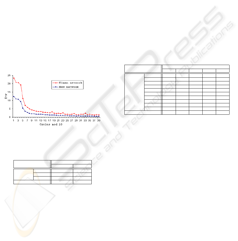
In order to compare the two networks, we trained
both networks on the same training set and tested
them on the same test set. The problem is to recognise
(classify) any input symbol into one of three symbols
used for this purpose. The learning rate was 0.1, mo-
mentum parameter was 0.02. The size of the training
set was 271×3 and the size of the test set was 472× 3
handwritten symbols. Our network is trained faster
and more stable because the generated mean square
errors, decrease faster and are smoother than Elman
network (see Figure 3); Our network generates higher
recognition rates than Elman network does (see Table
2). Note that the number of hidden units is 15 for both
networks. This corresponds to the minimum number
of hidden units for a recognition rate of 90% average
(B.Q. Huang and Kechadi, 2004).
Figure 3: The error tracks of trained Elman network and our
network
Table 2: The recognition rate of both networks for 3 digits
15 hidden neurons
Elman NET. new NET.
Digit 0 89.14 92.30
rec. 1 83.51 85.50
rate(%) 2 97.37 99.54
Ave. Rec Rate(%) 90.01 92.45
In this experiment we wanted to study the effect
of the number of hidden units on the network per-
formance on a bigger problem. The problem here is
to recognise a symbols between 0 to 9. The size of
the training set is 695 × 10 symbols taken from sec-
tion ”1a” in Unipen Train-R01/V07. The network is
trained step by step; e.g. for every 50 training cy-
cles we add another set of digits, until all the training
data has been added. The selected range of learning
rate is from 0.01 to 0.8, and the momentum range
is from 0.002 to 0.09. Their initial values are set to
the maximum allowed and during the training phase
they were decreased according to the learning algo-
rithm used. For instance, for the first 50 cycles of the
training phase, the learning rate is varied from 0.3 to
0.1, and the momentum is changed from 0.03 to 0.01.
Thus, the local minima are avoided, and the network
is trained faster.
The test set is of the same size of the training set
(695 × 10). The network with different layer con-
figurations is tested and the results are presented in
table 3. We notice that when the network used more
hidden units, the recognition rate is slightly higher.
This is because that the network has no control on
the pre-processing phase (feature extraction phase).
Some features were not optimised and therefore the
error is propagated to the network. When the features
are very represented the network achieves 100% ac-
curacy. We can notice also that 20 hidden neurons
are sufficient to reach an accuracy of 91% and a 40
hidden neurons to get an extra 5% accuracy.
Table 3: The recognition rate of each digit and the average
recognition rate of all the digits from each network config-
uration
Hidden neurons
20 25 30 35 40
0 92.80 95.68 94.10 95.54 96.26
1 90.93 93.38 93.52 95.10 94.10
2 88.20 91.94 91.08 96.40 96.12
Digit 3 92.09 95.25 97.98 96.12 96.98
Rec. 4 91.80 92.52 93.53 94.53 95.11
Rate 5 89.49 92.66 94.53 90.94 92.23
(%) 6 94.96 93.09 94.82 97.41 97.12
7 93.24 92.66 94.10 94.10 95.97
8 88.20 89.93 93.53 94.10 91.08
9 87.91 93.09 91.08 93.52 93.52
Ave. Rec Rate(%) 90.96 93.02 93.82 94.77 94.85
6 CONCLUSION & FUTURE
WORK
We presented an innovative approach for handwriting
recognition. This approach is composed of two main
techniques tackling different problems present in pat-
tern recognition applications. The first technique
deals with feature extraction, in which the output is
fed to the second which is the recognition process.
The first technique is based on fuzzy logic and the sec-
ond is a recurrent neural network, whose advantages
are strong discriminative power for pattern classifi-
cation and less computational overhead than RTRL.
This hybrid technique is proven to be very powerful
and efficient. In this paper we focussed on the second
process.
The network uses a dynamic learning algorithm
based on the gradient descent method. Experimen-
tal results, using benchmark datasets from Unipen,
show that the network is very efficient for a reason-
able number of hidden units. We believe that the
recognition rate will be improved if network architec-
ture is optimised and the features are generated taking
A RECURRENT NEURAL NETWORK RECOGNISER FOR ONLINE RECOGNITION OF HANDWRITTEN
SYMBOLS
33

into account the network architecture. There are also
some other issues that we will be our main focus in
the near future, such as the recognition of a bigger
set of symbols. The technique was implemented and
tested only for digits and we would like to study its
scalability with regards to the number of symbols to
be recognised and its computational overhead. Fur-
thermore, we will continue to explore and implement
different context layers and study their behaviour.
REFERENCES
B.Q. Huang, T. R. and Kechadi, T. (2004). A new mod-
ifed network based on the elman network. In Proc. of
IASTED Internation Conferance on Artificial Intelle-
gence and Application, Innsbruck, Austria.
C.C.Tappet (June 1984). Adaptive on-line handwriting
recognition. In Proc. 7th Int. conf. on Pattern Recog-
nition, pages 1004–1007, Montreal, Canada.
Elman, J. (1999). Finding structure in time. Cognitive Sci-
ence, 14(2):179–211.
Fausett, L. (1994). Fundamentals of Neural Networks. En-
glewood Cliffs, NJ: Prentice Hall.
Gomes, N. and Ling, L. L. (2001). Feature extraction based
on fuzzy set theory for handwriting recognition. In
ICDAR’01, pages 655–659.
Guyon, I., S. L. P. R. L. M. and Janet, S. (Oct, 1994).
Unipen project of on-line data exchange and recog-
nizer benchmarks. Proc. of the 12th International
Conference on Pattern Recognition,ICPR’94, pages
29–33.
J.A.Fitzgerald, F. and T.Kechadi (May 2004). Feature ex-
traction of handwritten symbols using fuzzy logic. In
The Seventeenth Canadian Conference on Artificial
Intelligence, pages 493–498.
J.Hu, M. and W.Turin (Oct, 1996). Hmm based on-line
handwriting recognition. IEEE Trans. Pattern Analy-
sis and Machine Intelligence, 18(10):1039–1045.
Lawrence, S., Giles, C. L., and Fong, S. (2000). Natural
language grammatical inference with recurrent neural
networks. IEEE Trans. on Knowledge and Data Engi-
neering, 12(1):126–140.
L.A.Zadeh (1972). Outline of a new approach to the analy-
sis of complex systems and decision processes. In
Man and Computer, pages 130–165.
L.R. Bahl, F. and Mercer, R. (March 1983). A maximum
likelihood approach to continuous speech recognition.
IEEE Trans. Pattern Analysis and Machine Intelli-
gence, 5(3):179–190.
M. Schnekel, I. G. and Henderson, D. (April 1994). On-line
cursive script recognition using time delay networks
and hidden markove models. In Proc. ICASSP’94,
volume 2, pages 637–640, Adelaide,Australia.
M.A. Castao, F. C. (1997). Training simple recurrent net-
works through gradient descent algorithms. In Lecture
Notes in Comp. Sci.: Biological & Artificial Computa-
tion: From Neuroscience to Technology, volume 1240,
pages 493–500. Springer Verlag.
Malaviya, A. and Peters, L. (1997). Fuzzy feature descrip-
tion of handwriting patterns. Pattern Recognition,
30(10):1591–1604.
O. D. Trier, A. K. J. and Taxt, T. (1996). Feature extrac-
tion methods for character recognition - a survey. In
Pattern Recognition, pages 641–662.
Plamondon, R. and Maarse, F. J. (May 1989). An evaluation
of motor models of handwriting. IEEE Trans. systems
Man, and Cybernetics, 19:1060–1072.
Rabiner, L. (Feb 1989). A tutorial on hidden markov models
and selected applications in speech recognition. Proc.
of the IEEE, 77(2).
R.J.Williams and Zipser, D. (1995). Gradient-based learn-
ing algorithms for recurrent networks and their com-
putational complexity. In Chauvin, Y. and Rumelhart,
D. E., editors, Back-propagation: Theory, Architec-
tures and Applications, chapter 13, pages 433–486.
Lawrence Erlbaum Publishers, Hillsdale, N.J.
S. Bercu, G. L. (May 1993). On-line handwritten word
recognition: An approach based on hidden markov
models. In Proc. 3r Int.Workshop on frontiers in
Handwriting Recognition, pages 385–390, buffalo,
New York.
Schomaker, L. R. B. and Tteulings, H.-L. (April 1990). A
handwriting recognition system based on the prop-
erties and architectures of the human motor system.
In Proc. Int. Workshop on frontiers in Handwriting
Recognition, Montreal, pages 195–211.
S.E. Levinson, L. R. and Sondhi, M. (April 1983). An into
the application of the theory of probabilistic functions
of a markov process to automatic speech recognition.
Bell System Technical Joural, 62(4):1035–1074.
Seni, G. and Nasrabadi, N. (1994). An on-line cursive word
recognition system. In CVPR94, pages 404–410.
Subrahmonia, J. and Zimmerman, T. (2000). Pen comput-
ing: Challenges and applications. In Proc. ICPR 2000,
pages 2060–2066.
T.Wakahara and K.Odaka (Dec. 1997). On-line cursive
kanji character recognition using stroke-based afine
transformation. IEEE Trans. Pattern Analysis and Ma-
chine Intelligence, 19(12).
Werbos, P. J. (1990). Backpropagation through time: what
it does and how to do it. In Proc. of the IEEE, vol-
ume 78, pages 1550–1560.
Williams, R. and Zipser, D. (1989). A learning algo-
rithm for continually running fully recurrent neural
networks. Neural Computation, 1(2):270–280.
Wilson, W. H. (1996). Learning performance of networks
like elman’s simple recurrent netwroks but having
multiple state vectors. Workshop of the 7th Australian
Conference on Neural Networks, Australian National
University Canberra.
Zadeh, L. (1975). Calculus of fuzzy restrictions. In Fuzzy
Sets and Their Applications to Cognitive and Decision
Processes, pages 1–39, Academic Press, NY.
ICEIS 2005 - ARTIFICIAL INTELLIGENCE AND DECISION SUPPORT SYSTEMS
34
