MINING VERY LARGE DATASETS WITH SVM AND
VISUALIZATION
Thanh-Nghi Do, François Poulet
ESIEA Recherche, BP 0339, 53003 Laval-France
Keywords: Mining very large datasets, Support vector machines, Active
learning, Interval data analysis, Visual data
mining, Information visualization.
Abstract: We present a new support vector machine (SVM) algorithm and graphical methods for mining very large
datasets. We develop the active selection of training data points that can significantly reduce the training set
in the SVM classification. We summarize the massive datasets into interval data. We adapt the RBF kernel
used by the SVM algorithm to deal with this interval data. We only keep the data points corresponding to
support vectors and the representative data points of non support vectors. Thus the SVM algorithm uses this
subset to construct the non-linear model. We also use interactive graphical methods for trying to explain the
SVM results. The graphical representation of IF-THEN rules extracted from the SVM models can be easily
interpreted by humans. The user deeply understands the SVM models’ behaviour towards data. The
numerical test results are obtained on real and artificial datasets.
1 INTRODUCTION
The SVM algorithms proposed by (Vapnik, 1995)
are a well-known class of data mining algorithms
using the idea of kernel substitution. SVM and
kernel related methods have shown to build accurate
models. They have shown practical relevance for
classification, regression or novelty detection.
Successful applications of SVM have been reported
for various fields, for example in face identification,
text categorization, bioinformatics (Guyon, 1999).
SVM and kernel methodology have become
increasingly popular data mining tools. Although the
prominent properties of SVM, they are not
favourable to deal with the challenge of large
datasets. SVM solutions are obtained from quadratic
programs (QP) possessing a global solution, so that,
the computational cost of an SVM approach is at
least square of the number of training data points
and the memory requirement makes SVM
impractical. The effective heuristics to scale up
SVM learning task are to divide the original QP into
series of small problems (Boser et al., 1992), (Osuna
et al., 1997), (Platt, 1999), incremental learning
(Syed et al., 1999), (Fung and Mangasarian, 2002)
updating solutions in growing training set, parallel
and distributed learning (Poulet and Do, 2004) on
personal computer (PC) network or choosing
interested data points subset (active set) for learning
(Tong and Koller, 2000).
While SVM gives good results, the interpretation of
these res
ults is not so easy. The support vectors
found by the algorithms provide limited information.
Most of the time, the user only obtains information
regarding the support vectors being used as “black
box” to classify the data with a good accuracy. It is
impossible to explain or even understand why a
model constructed by SVM performs a better
prediction than many other algorithms. Therefore, it
is necessary to improve the comprehensibility of
SVM models. Very few papers have been published
about methods trying to explain SVM results
(Caragea et al., 2001), (Poulet, 2004).
Our investigation aims at scaling up SVM
al
gorithms to mine very large datasets and using
graphical tools to interpret the SVM results.
We develop the active learning algorithm that can
sig
nificantly reduce the training set in the SVM
classification. Large datasets are aggregated into
smaller datasets using interval data concept (one
kind of symbolic data (Bock and Diday, 1999)). We
adapt the RBF kernel used by the SVM algorithm to
127
Do T. and Poulet F. (2005).
MINING VERY LARGE DATASETS WITH SVM AND VISUALIZATION.
In Proceedings of the Seventh International Conference on Enterprise Information Systems, pages 127-134
DOI: 10.5220/0002548601270134
Copyright
c
 SciTePress

deal with these interval data. We only keep the data
points corresponding to support interval vectors and
the representative data points of non support interval
vectors. Thus the SVM algorithm uses this subset to
construct the non-linear model. Our algorithm can
deal with one million data points in minutes on one
personal computer.
We also use interactive graphical methods for trying
to explain the SVM results. The interactive decision
tree algorithms (Ankerst et al., 1999), (Poulet, 2002)
involve the user in the construction of decision tree
models on prediction results obtained at the SVM
output. The SVM performance in classification task
is deeply understood in the way of the IF-THEN
rules extracted intuitively from the graphical
representation of the decision trees that can be easily
interpreted by humans. The comprehensibility of
SVM models is significantly improved.
This paper is organized as follows. In section 2, we
briefly present SVM algorithm. Section 3 describes
our active SVM algorithm that is used to deal with
very large datasets. In section 4, we present the
inductive rule extraction method for interpreting the
SVM result. We demonstrate numerical test results
in section 5 before the conclusion and future works
in section 6.
2 SVM ALGORITHM
Let us consider a binary linear classification task, as
depicted in figure 1, with m data points x
1
, x
2
, …, x
m
in a n-dimensional input having corresponding
labels y
i
= ±1.
SVM algorithm aims to find the best separating
plane (represented by the vector w and the scalar b)
as being furthest from both classes. It can
simultaneously maximize the margin between the
support planes for each class and minimize the error.
This can also be accomplished through the quadratic
program (1):
Min (1/2)||w||
2
+ C
∑
=
m
i
i
z
1
s.t. y
i
( w.x
i
– b ) + z
i
≥ 1 (1)
where the slack variable z
i
≥ 0 (i=1,..,m) and C is a
positive constant used to tune the margin and the
error.
margin = 2/||w||
w.x – b = +1
w.x – b = –1
optimal plane:
w.x – b = 0
+1
-1
z
i
margin = 2/||w||
w.x – b = +1
w.x – b = –1
optimal plane:
w.x – b = 0
+1
-1
z
i
Figure 1: Linear binary classification with SVM
The dual Lagrangian of the quadratic program (1) is:
Min (1/2)
–
∑∑
==
m
i
m
j
jijiji
xxyy
11
. αα
∑
=
m
i
i
1
α
s.t.
= 0 (2)
∑
=
m
i
ii
y
1
α
C ≥ α
i
≥ 0 (i = 1,…,m)
From the α
i
obtained by the solution of (2), we can
recover the plane:
w =
∑
and the scalar b determined by the
support vectors (for which α
=
SV
i
iii
xy
#
1
α
i
> 0).
And then, the classification function of a new data
point x based on the plane is: sign (w.x – b)
To change from a linear to nonlinear classification,
no algorithmic changes are required from the linear
case other than substitution of a kernel evaluation
ICEIS 2005 - ARTIFICIAL INTELLIGENCE AND DECISION SUPPORT SYSTEMS
128

for the simple dot product of (2). And then, it can be
tuned into a general nonlinear algorithm:
Min (1/2)
–
∑
∑∑
==
m
i
m
j
jijiji
xxKyy
11
),( αα
=
m
i
i
1
α
s.t.
= 0 (3)
∑
=
m
i
ii
y
1
α
C ≥ α
i
≥ 0 (i = 1,…,m)
By changing the kernel function K as a polynomial
or a radial basis function, or a sigmoid neural
network, we can get different nonlinear
classification. The classification of a new data point
x is based on:
sign(
– b) (4)
∑
=
SV
i
iii
xxKy
#
1
),( α
SVM algorithms solve the QP (3) being well known
at least square of the number of training data points
and the memory requirement is expensive. The
practical implement methods including chunking,
decomposition (Boser et al., 1992), (Osuna et al.,
1997) and sequence minimal optimization (Platt,
1999) divide the original QP into series of small
problems.
Incremental proximal SVM proposed by (Fung and
Mangasarian, 2002) is another SVM formulation
very fast to train because it requires only the solution
of a linear system. This algorithm only loads one
subset of the data at any one time and updates the
model in incoming training subsets. The authors
have performed the linear classification of one
billion data points in 10-dimensional input space
into two classes in less than 2 hours and 26 minutes
on a Pentium II.
Some parallel and distributed incremental SVM
algorithms (Poulet and Do, 2004) or boosting of
SVM (Do and Poulet, 2004a) can deal with at least
one billion data points on PCs in some minutes.
Active learning algorithms (Tong and Koller, 2000)
only use data points closest to the separating plane.
These algorithms can deal with either very large
datasets in linear classification problem or non linear
classification on medium datasets (in tens of
thousands data points).
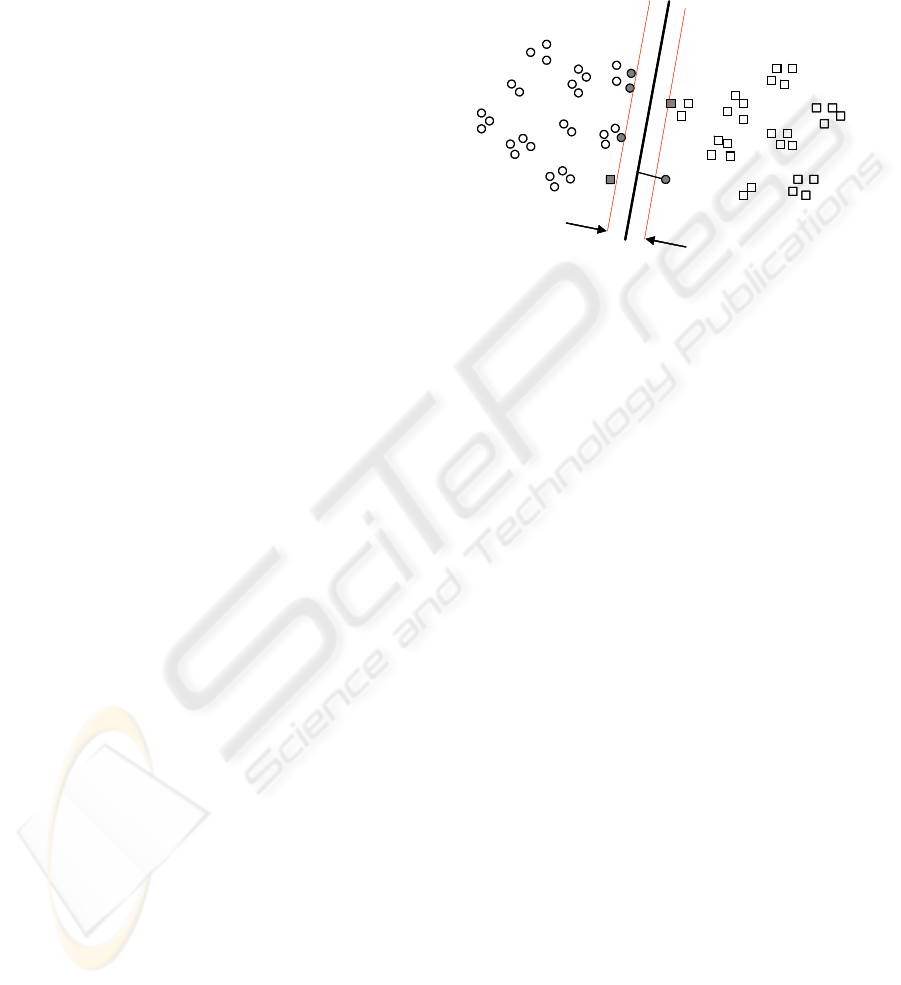
3 ACTIVE SVM FOR LARGE
DATASETS
w.x – b = 0
+1
-1
w.x – b = 0
+1
-1
Active subset
selection
w.x – b = 0
+1
-1
w.x – b = 0
+1
-1
w.x – b = 0
+1
-1
w.x – b = 0
+1
-1
Active subset
selection
Figure 2: SVM learning on active subset
Our active SVM algorithm exploits the separating
boundary structure which only depends on training
data points closed (support vectors) to it, thick points
as depicted in figure 2. The natural clusters of these
training data points also relate to the decision
boundary of SVM. Therefore, our algorithm selects
the clusters closed to the separating boundary. We
summarize large datasets into clusters. The SVM
algorithm is trained on clusters, we obtain the
support vectors at the output containing data points
for creating the separating boundary. However, we
MINING VERY LARGE DATASETS WITH SVM AND VISUALIZATION
129

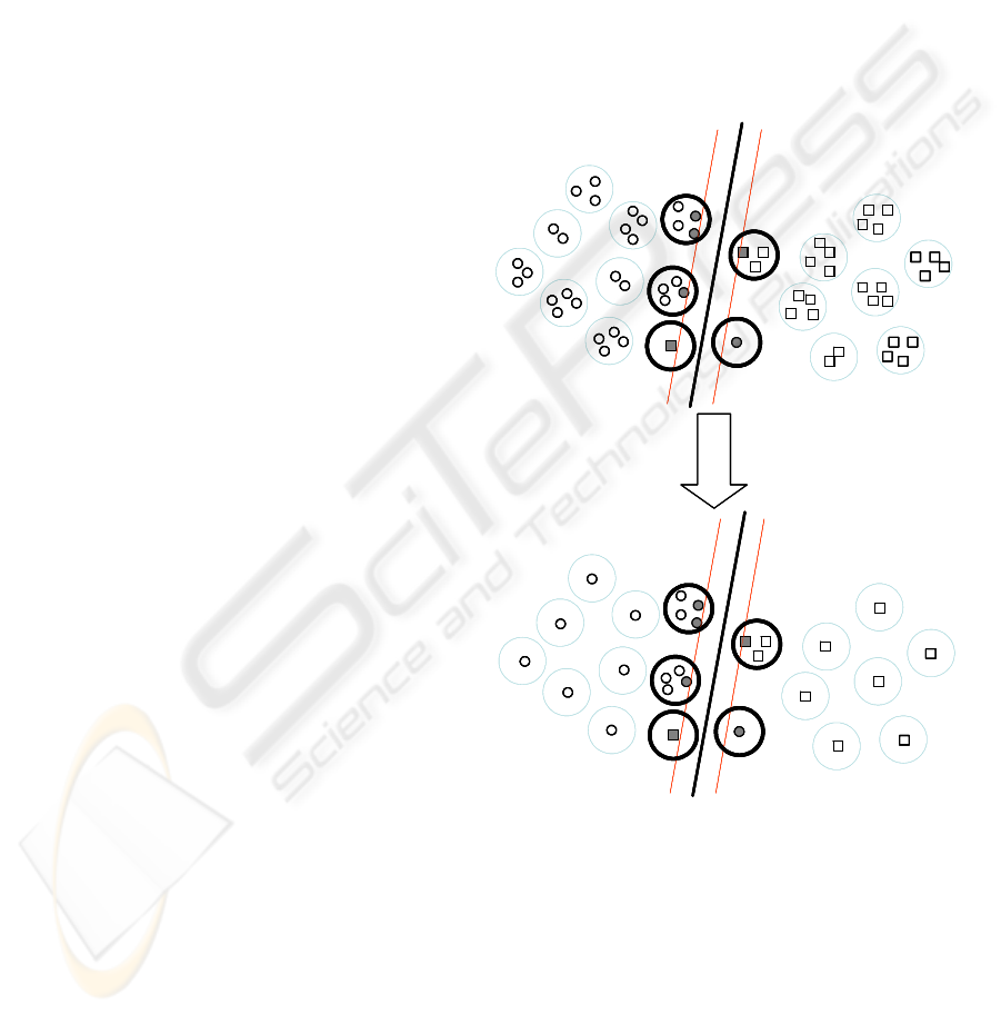
need to adapt SVM on high level data clusters. If the
clusters are represented by their centers, we can lose
information. So that, we use the interval data
concept to represent the clusters. A interval vector
corresponds to a cluster, the low and high values of
an interval are computed by low and high bound of
data points in this cluster. After that, we construct
non linear kernel function RBF for dealing with
interval datasets.
Figure 3: Optimal planes based on cluster centers and
interval data
3.1 Active selection for SVM using
interval data concept
K(x,y) =
⎟
⎟
⎠
⎞
⎜
⎜
⎝
⎛
−−
2
2
2
exp
σ
yx
(5)
Assume we have two data points x and y ∈ R
n
, the
RBF kernel formula in (5) of two data vectors x and
y of continuous type is based on the Euclidean
distance between these vectors, d
E
(x,y) = ||x – y||.
For dealing with interval data, we only need to
measure the distance between two vectors of interval
type, after that we substitute this distance measure
for the Euclidean distance into RBF kernel formula.
Thus the new RBF kernel can deal with interval
data. The popular known dissimilarity measure
between two data vectors of interval type is the
Hausdorff (1868-1942) distance.
Suppose that we have two intervals represented by
low and high values: I
1
= [low
1
, high
1
] and I
2
=
[low
2
, high
2
], the Hausdorff distance between two
intervals I
1
and I
2
is defined by formula (6):
d
H
(I
1
, I
2
) = max(|low
1
– low
2
|, |high
1
– high
2
|) (6)
Let us consider two data vectors u, v ∈ Ω having n
dimensions of interval type:
u = ([u
1,low
, u
1,high
], [u
2,low
, u
2,high
],…, [u
n,low
, u
n,high
]),
v = ([v
1,low
, v
1,high
], [v
2,low
, v
2,high
],…, [v
n,low
, v
n,high
]).
optimal plane for
interval data
optimal plane for
cluster centers
optimal plane for
interval data
optimal plane for
cluster centers
The Hausdorff distance between two vectors u and v
is defined by formula (7):
d
H
(u, v) =
()
∑
=
−−
n
i
highihighilowilowi
vuvu
1
2
,,,,
,max
(7)
By substituting the Hausdorff distance measure d
H
into RBF kernel formula, we obtain a new RBF
kernel for dealing with interval data. This
modification tremendously changes SVM algorithms
for mining interval data. No algorithmic changes are
required from the habitual case of continuous data
other than the modification of the RBF kernel
evaluation. All the benefits of the original SVM
methods are maintained. We can use SVM
algorithms to build interval data mining models in
classification, regression and novelty detection. We
only focus on the classification problem.
3.2 Algorithm description
We obtain the support interval vectors from learning
task on high level representative clusters. We create
the active learning subset by extracting data points
from the support interval vectors and getting some
representative data points of non support interval
vectors. This active subset is used to construct the
SVM model. The active learning algorithm is
described in table 1. The large dataset is drastically
reduced. The algorithm with RBF kernel can classify
one million data points in an acceptable execution
time (11 hours for creating the clusters and selecting
the active learning and 17.69 seconds for
constructing the SVM model) on one PC (Pentium-
4, 2.4 GHz, 512 MB RAM).
ICEIS 2005 - ARTIFICIAL INTELLIGENCE AND DECISION SUPPORT SYSTEMS
130

Table 1: Active SVM algorithm
4 INTERPRET SVM RESULTS
Although SVM algorithms have shown to build
accurate models, their results are very difficult to
understand. Most of the time, the user only obtains
information regarding the support vectors being used
as “black box” to classify the data with a good
accuracy. The user does not know how SVM models
can work. For many data mining applications,
understanding the model obtained by the algorithm
is as important as the accuracy, it is necessary that
the user has confidence in the knowledge discovered
(model) by data mining algorithms. (Caragea et al.,
2001) proposed to use Grand Tour method (Asimov,
1985) to try to visualize support vectors. The user
can see the separating boundary between two
classes. (Poulet, 2004), (Do and Poulet, 2004b) have
combined some strengths of different visualization
methods to visualize the SVM results. These
methods can detect and show interesting dimensions
in the obtained model.
We propose here to use interactive decision tree
algorithms, PBC (Ankerst et al, 1999) or CIAD
(Poulet, 2002) to try to explain the SVM results. The
SVM performance in classification task is deeply
understood in the way of IF-THEN rules extracted
intuitively from the graphical representation of the
decision trees that can be easily interpreted by
humans.
Input: dataset S = {positive data points (P),
negative data points (
N)}
Output: a classification function
f
Training:
1. Summarize dataset
S into interval data IS =
{interval positive data points, interval negative
data points} using clustering algorithms,
2. Select support interval vectors (
SIV) using
SVM algorithm with non linear RBF kernel
function constructed in interval data:
SIV = SVM_train(IS)
3. Active learning dataset
AS created by
getting representative data points of non
support interval vectors and extracting data
points from support interval vectors
SIV.
4. Construct SVM model with the RBF kernel
function on active learning dataset
AS:
f = SVM_train(AS)
Table 2: Inductive rule extraction from SVM models
Input: non label dataset SP et a SVM
classification function
f
Output: inductive rule set
IND-RULE
Extracting:
1. Classify non label dataset
SP using SVM
classification function
f, we obtain label set L
assigned to
SP:
{
SP, L} = SVM_classify(SP, f)
2. Interactively constructing decision tree
model
DT on dataset {SP, L} using visual
data mining decision tree algorithms, i.e. PBC
(Ankerst et al, 1999) or CIAD (Poulet, 2002).
3. User extracts inductive rules
IND-RULE
from graphical representation of decision tree
model
DT:
IND-RULE = HumanExtract(graphical DT)
The rule extraction prototype is described in table 2.
We classify dataset using the SVM model, after that
the user constructs the decision tree model on the
obtained result (dataset and classes predicted by the
SVM models). Thus he can easily extract inductive
rules from graphical representation of the decision
tree model. The SVM models are understood in the
way of IF-THEN rules that facilitate human
interpretation.
We propose to use the visual data mining decision
tree algorithms because they involve more
intensively the user in the model construction using
interactive visualization techniques. This can help
the user to improve the comprehensibility of the
obtained model, and thus his confidence in the
knowledge discovered is increased.
For example, the SVM algorithm using a RBF
kernel separates class 1-against-all in the Segment
MINING VERY LARGE DATASETS WITH SVM AND VISUALIZATION
131

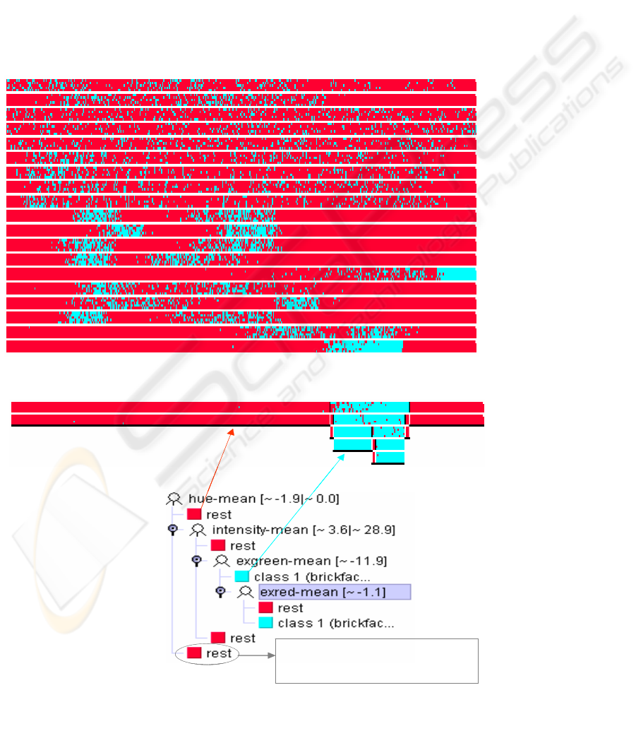
Dataset (Michie et al., 1994) having 2310 data
points in 19 dimensions with 99.56 % accuracy.
PBC uses bars to visualize the result at the SVM
output (cf. figure 4). Each bar represents one
independent dimension. Within it, the values of one
dimension are sorted and mapped to pixels (colour =
class) in line-by-line according to their order. The
user interactively chooses the best separating split to
construct the decision tree (based on the human
pattern recognition capabilities) or with the help of
automatic algorithms. The obtained decision tree (cf.
figure 5) having 7 rules can explain 99.80 %
performance of the SVM model. One rule is created
for each path from the root to a leaf, each dimension
value along a path forms a conjunction and the leaf
node holds the class prediction. And thus, the non
linear SVM is interpreted in the way of the 7
inductive rules (IF-THEN) that will be easily
understood by humans.
Rule 1: IF (hue-mean < -1.9) THEN CLASS = rest
(non brickface)
Rule 2: IF ((-1.9 <= hue-mean < 0.0) and (intensity-
mean < 3.6)) THEN CLASS = rest
Rule 3: IF ((-1.9 <= hue-mean < 0.0) and (3.6 <=
intensity-mean < 20.9) and (exgreen-mean < -11.9)
and (exred-mean < -1.1)) THEN CLASS = brickface
region-centroid-col
region-centroid-row
region-pixel-count
short-line-density-5
short-line-density-2
vedge-mean
vegde-sd
hegde-mean
hegde-sd
intensity-m ean
rawred-mean
rawblue-mean
rawgreen-mean
exred-mean
exblue-mean
exgreen-mean
value-mean
saturation-m ean
hue-mean
IF (hue-mean < -1.9) TH EN
CLASS = non brickface
Figure 4: Visualization with PBC of the SVM result on the Segm ent Dataset (1-against-all)
Figure 5: Visualization of the decision tree explaining the SVM result on the Segment Dataset
region-centroid-col
region-centroid-row
region-pixel-count
short-line-density-5
short-line-density-2
vedge-mean
vegde-sd
hegde-mean
hegde-sd
intensity-m ean
rawred-mean
rawblue-mean
rawgreen-mean
exred-mean
exblue-mean
exgreen-mean
value-mean
saturation-m ean
hue-mean
region-centroid-col
region-centroid-row
region-pixel-count
short-line-density-5
short-line-density-2
vedge-mean
vegde-sd
hegde-mean
hegde-sd
intensity-m ean
rawred-mean
rawblue-mean
rawgreen-mean
exred-mean
exblue-mean
exgreen-mean
value-mean
saturation-m ean
hue-mean
IF (hue-mean < -1.9) TH EN
CLASS = non brickface
IF (hue-mean < -1.9) TH EN
CLASS = non brickface
Figure 4: Visualization with PBC of the SVM result on the Segm ent Dataset (1-against-all)
Figure 5: Visualization of the decision tree explaining the SVM result on the Segment Dataset
Figure 4: Visualization with PBC of the SVM result on the Segment Database (1-against-all)
Figure 5: Visualization of the decision tree explaining the SVM result on the Segment Database
ICEIS 2005 - ARTIFICIAL INTELLIGENCE AND DECISION SUPPORT SYSTEMS
132

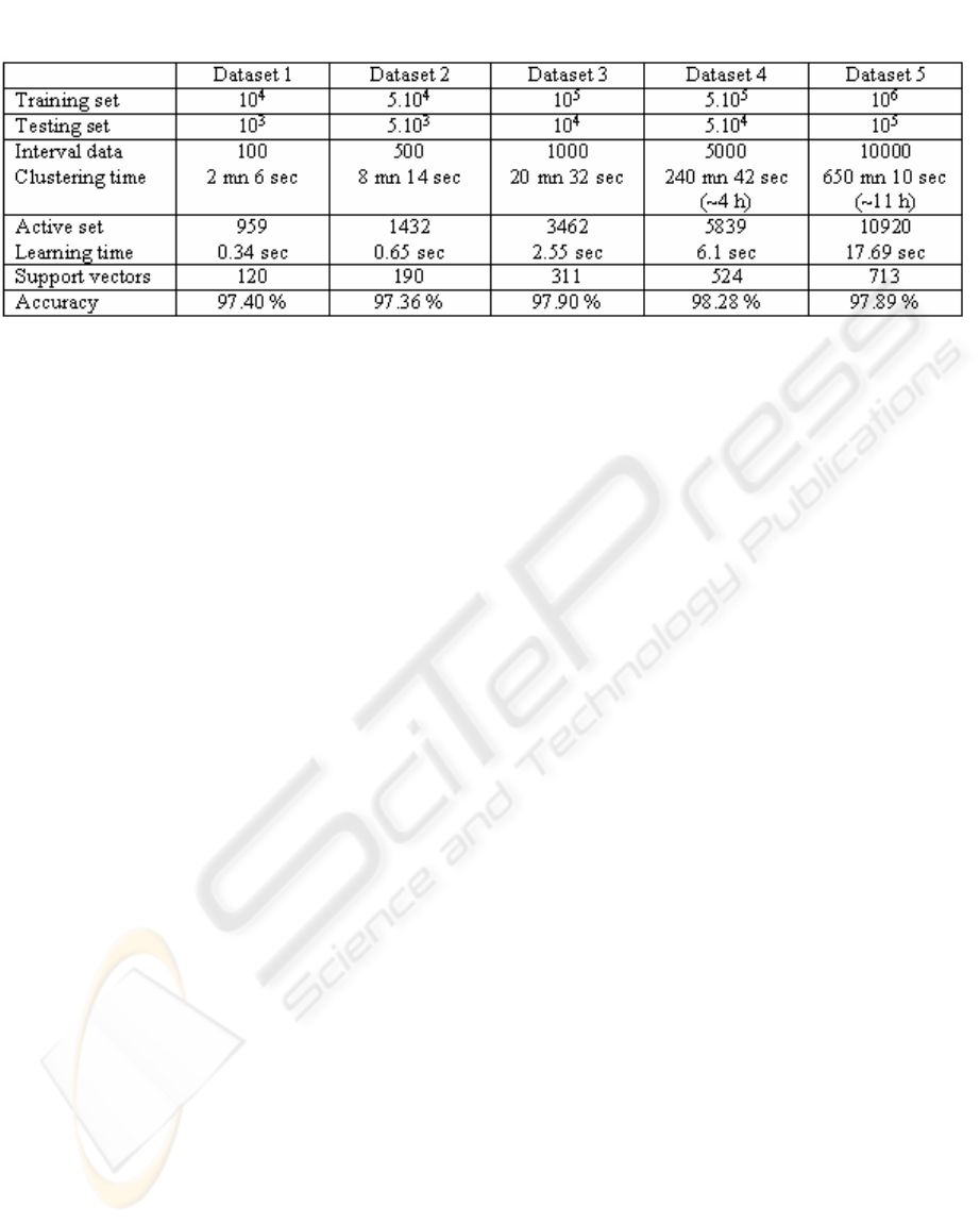
Tab tsle 3: Classification results on large dataseTab tsle 3: Classification results on large datase
Table 3: Classification results on large datasets.
Rule 4: IF ((-1.9 <= hue-mean < 0.0) and (3.6 <=
intensity-mean < 20.9) and (exgreen-mean < -11.9)
and (exred-mean >= -1.1)) THEN CLASS = rest
Rule 5: IF ((-1.9 <= hue-mean < 0.0) and (3.6 <=
intensity-mean < 20.9) and (exgreen-mean >= -
11.9)) THEN CLASS = brickface
Rule 6: IF ((-1.9 <= hue-mean < 0.0) and (intensity-
mean >= 20.9)) THEN CLASS = rest
Rule 7: IF (hue-mean >= 0.0) THEN CLASS = rest
The user uses these rules for interpreting the
performance of the SVM model. This can help him
to deeply understand how the SVM algorithm can
work.
5 NUMERICAL TEST RESULTS
To evaluate the performance of our active SVM
algorithm on very large datasets, we have added to
the publicly available toolkit, LibSVM (Chang and
Lin, 2003) a new code of the RBF kernel for dealing
with interval data. Thus, the software program is
able to deal with both interval and continuous data in
classification. We focus on numerical tests with
large datasets (cf. table 3) generated by the
RingNorm program from (Delve, 1996). It is a 20
dimensional, 2 class classification example. Each
class is drawn from a multivariate normal
distribution. Class 1 has mean zero and covariance 4
times the identity. Class 2 has mean (m, m, …, m)
and unit covariance with m = 2/sqrt(20). We use one
Pentium-4, 2.4 GHz, 512 MB RAM running Linux
Redhat 9.0 for all experiments. In the simple way,
the large datasets are aggregated into smaller ones
(interval data) using the K-means algorithm
(MacQueen, 1967). (Bock and Diday, 1999)
proposed many methods for this problem.
The results obtained by SVM with the RBF kernel
function in table 3 show that our active SVM
algorithm chooses efficiently the active learning sets
in large datasets for training SVM models.
Therefore, the learning time and memory
requirement are drastically reduced. Thus the
algorithm is able to deal with non linear
classification in massive datasets (10
6
data points)
on one personal computer in acceptable execution
time.
6 CONCLUSION
We have developed a new active SVM algorithm for
mining very large (10
6
data points) datasets on
personal computers. The main idea is to choose the
active training data points that can significantly
reduce the training set in the SVM classification. We
summarize the massive datasets into interval data.
We adapt the RBF kernel used by the SVM
algorithm to deal with thisinterval data. We only
keep the data points corresponding to support
vectors and the representative data points of non
support vectors. Thus the SVM algorithm uses this
subset to construct the non-linear model with good
results.
We also propose to use interactive decision tree
algorithms for trying to explain the SVM results.
The user can interpret the SVM performance in
classification task in the way of IF-THEN rules
extracted intuitively from the graphical
representation of the decision trees that can be easily
interpreted by humans.
The first future work will be to use high level
representative data for searching the SVM
parameters. This approach drastically reduces the
cost compared with the research in initial large
datasets.
MINING VERY LARGE DATASETS WITH SVM AND VISUALIZATION
133

Another one will be to extend our approach
combining visualization methods and automatic
algorithms for mining very large datasets and
interpreting the results too.
REFERENCES
Ankerst, M., Elsen, C., Ester, M., and Kriegel, H-P., 1999,
“Visual Classification: An Interactive Approach to
Decision Tree Construction”, in proc. of Proceeding of
the 5
th
ACM SIGKDD Int. Conf. on KDD’99, San
Diego, USA, pp. 392-396.
Asimov, D., 1985, “The Grand Tour: A Tool for Viewing
Multidimensional Data”, in SIAM Journal on
Scientific and Statistical Computing, 6(1), pp. 128-
143.
Bennett, K., and Campbell, C., 2000, “Support Vector
Machines: Hype or Hallelujah?”, in SIGKDD
Explorations, Vol. 2, No. 2, pp. 1-13.
Bock, H-H., and Diday, E., 1999, “Analysis of Symbolic
Data”, Springer-Verlag.
Boser, B., Guyon, I., and Vapnik, V., 1992, “An Training
Algorithm for Optimal Margin Classifiers”, in Fifth
ACM Annual Workshop on Computational Learning
Theory, Pittsburgh, Pennsylvania, pp. 144-152.
Caragea, D., Cook, D., and Honavar, V., 2001, “Gaining
Insights into Support Vector Machine Pattern
Classifiers Using Projection-Based Tour Methods”, in
proc. the 7
th
ACM SIGKDD Int. Conf. on KDD’01,
San Francisco, USA, pp. 251-256.
Chang, C-C., and Lin, C-J., 2003, “A Library for Support
Vector Machines”, http://www.csie.ntu.edu.tw/~cjlin/-
libsvm
Delve, 1996, “Data for Evaluating Learning in Valid
Experiments”, http://www.cs.toronto.edu/~delve
Do, T-N., and Poulet, F., 2004a, “Towards High
Dimensional Data Mining with Boosting of PSVM
and Visualization Tools”, in proc. of ICEIS’04, 6
th
Int.
Conf. on Entreprise Information Systems, Vol. 2, pp.
36-41, Porto, Portugal.
Do, T-N., and Poulet, F., 2004b, “Enhancing SVM with
Visualization”, in Discovery Science 2004, E. Suzuki
et S. Arikawa Eds., Lecture Notes in Artificial
Intelligence 3245, Springer-Verlag, pp. 183-194.
Fung, G., and Mangasarian, O., 2002, “Incremental
Support Vector Machine Classification”, in proc. of
the 2
nd
SIAM Int. Conf. on Data Mining SDM'2002
Arlington, Virginia, USA.
Guyon, I., 1999, “Web Page on SVM Applications”,
http://www.clopinet.com/isabelle/Projects/SVM/app-
list.html
MacQueen, J., 1967, “Some Methods for classification
and Analysis of Multivariate Observations”, in proc.
of 5
th
Berkeley Symposium on Mathematical Statistics
and Probability, Berkeley, University of California
Press, Vol. 1, pp. 281-297.
Michie, D., Spiegelhalter, D-J., and Taylor, C-C., 1994,
“Machine Learning, Neural and Statistical
Classification”, Ellis Horwood.
Osuna, E., Freund, R., and Girosi, F., 1997, “An Improved
Training Algorithm for Support Vector Machines”, in
Neural Networks for Signal Processing VII, J.
Principe, L. Gile, N. Morgan, and E. Wilson Eds., pp.
276-285.
Platt, J., 1999, “Fast Training of Support Vector Machines
Using Sequential Minimal Optimization”, in Advances
in Kernel Methods -- Support Vector Learning, B.
Schoelkopf, C. Burges, and A. Smola Eds., pp. 185-
208.
Poulet, F., 2002, “Full-View: A Visual Data Mining
Environment”, Int. Journal of Image and Graphics,
2(1), pp. 127-143.
Poulet, F., 2004, “Towards Visual Data Mining”,in proc.
of ICEIS’04, 6
th
Int. Conf. on Entreprise Information
Systems, Vol. 2, pp. 349-356, Porto, Portugal.
Poulet, F., and Do, T-N., 2004, “Mining Very Large
Datasets with Support Vector Machine Algorithms”,
in Enterprise Information Systems V, O. Camp, J.
Filipe, S. Hammoudi et M. Piattini Eds., Kluwer
Academic Publishers, 2004, pp. 177-184.
Syed, N., Liu, H., and Sung, K., 1999, “Incremental
Learning with Support Vector Machines”, in proc. of
the 6
th
ACM SIGKDD Int. Conf. on KDD'99, San
Diego, USA.
Tong, S., and Koller, D., 2000, “Support Vector Machine
Active Learning with Applications to Text
Classification”, in proc. of ICML’00, the 17
th
Int.
Conf. on Machine Learning, Stanford, USA, pp. 999-
1006.
Vapnik, V., 1995, “The Nature of Statistical Learning
Theory”, Springer-Verlag, New York.
ICEIS 2005 - ARTIFICIAL INTELLIGENCE AND DECISION SUPPORT SYSTEMS
134