
A Multi-Resolution Learning Approach to Tracking
Concept Drift and Recurrent Concepts
Mihai M. Lazarescu
Faculty of Computer Science, Curtin University,
GPO Box U1987, Perth 6001, W.A.
Abstract. This paper presents a multiple-window algorithm that combines a
novel evidence based forgetting method with data prediction to handle different
types of concept drift and recurrent concepts. We describe the reasoning behind
the algorithm and we compare the performance with the FLORA algorithm on
three different problems: the STAGGER concepts problem, a recurrent concept
problem and a video surveillance problem.
1 Introduction
Incremental learning is used more and more often today across many domains. The
reason for the increased focus on incremental learning techniques is that the learning
is dynamic and hence it is more applicable to real world situations such as on-line
processing or mining large datasets. An important issue of incremental learning which
this work addresses is that of tracking and adapting to changes in the data, specifically
we refer to the problem of concept drift. A brief definition of the problem of concept
drift is as follows: “In many real-world domains, the context in which some concepts
of interest depend may change, resulting in more or less abrupt and radical changes
in the definition of the target concept. The change in the target concept is known as
concept drift” [8]. The main difficulty in tracking concept drift is that there is no prior
knowledge of the type, pace and timing of the change that is likely to occur. Hence
model based or time series based approaches are not suited for this problem.
A crucial aspect of the concept drift problem is forgetting. The algorithms developed
to handle concept drift generally use a time based mechanism to control the forgetting
process which generally leads to two problems: useful information is being discarded
and the system converges more slowly to the target concept. Furthermore, the systems
simply react to changes rather than attempt to predict and classify the changes in the
data.
This paper presents a multiple window approach to track different types of concept
drift. The algorithm attempts to interpret current data as well as detect, predict and
quickly adapt to future changes in the concept. The system is designed to work in an
on-line scenario where the data consists of a sequential stream of examples which are
used by the system to derive a concept description that is consistent with the information
observed.
The work presented makes three novel contributions. The first novel aspect of the
research is that the algorithm uses a usefulness based approach to control the forgetting
M. Lazarescu M. (2005).
A Multi-Resolution Learning Approach to Tracking Concept Drift and Recurrent Concepts.
In Proceedings of the 5th International Workshop on Pattern Recognition in Information Systems, pages 52-62
DOI: 10.5220/0002568900520062
Copyright
c
SciTePress

mechanism used to discard data from the system’s memory. Rather than using a time
based approach, the forgetting mechanism analyses the newly observed data instance
to determine how well it fits with the rest of the instances in the system’s memory and
the current concept definition. Based on the the rest of the data, the mechanism also
determines if the new instance is a likely indicator of a change in the concept. Once the
usefulness of the instance has been estimated, the system checks both the usefulness and
age of the instance to determine whether or not the the instance is to be discarded. The
second contribution is that the algorithm predicts the rate of change to give the system a
pro-active approach to the data and thus improve the accuracy of the concept tracking.
The algorithm consistently checks the current rate of change and estimates (based on
past history) what the future rate of change is likely to be. This information is used to
improve the control over the size of the larger dynamic data window which acts as the
memory of the system and it allows for a faster adaptation to changes in the concept.
The third contribution is the representation used for the concepts tracked. Rather than
storing a simple generalization of the data observed, we represent the concept through a
combination of instance generalizations, data predictors and the rate of change observed
when concept was stable. Moreover, we use a knowledge repository to store old concept
descriptions to avoid having to “re-learn” recurrent concepts.
2 Related Work
The issue of concept drift has been investigated for many years and several systems
have been developed to address the problem of concept drift. The aim of the research
in this area is to develop algorithms that will allow a system to adapt concepts quickly
to permanent change while avoiding any unncessary changes if the change observed is
determined to be virtual (temporal) or noise.
The first system developed to deal with concept drift was STAGGER [7]. The learn-
ing method employed by STAGGER is based on a concept representation which uses
symbolic characterizations that have a sufficiency and a necessity weight associated
with them. As the system processes the data instances, it either adjusts the weights
associated with the characterizations or it creates new ones.
The FLORA family of algorithms implements a moving window approach to deal
with concept drift [9, 2]. FLORA2 is a supervised incremental learning system that
uses a stream of positive and negative examples to track concepts that change over
time. FLORA2 has a heuristic routine to dynamically adjust its window size and uses a
better generalization technique to integrate the knowledge extracted from the examples
observed. FLORA2 has been improved first by adding new routines to better handle
noise (FLORA3) and to handle the issue of recurring contexts (FLORA4).
A different approach to dealing with concept drift was used in the AQ-PM [5] and
SPLICE [1] batch learning systems. AQ-PM is a partial memory system, [5, 6,4]. The
system analyzes the training instances and selects only “extreme examples” which it
deems to lie at the extremities of concept descriptions. SPLICE [1] is an off-line meta-
learning system that uses contextual clustering to deal with concept drift that occurs as
a result of hidden changes in contexts. The learning process assumes that some con-
53

sistency exists in the data and the system groups together sequences of instances into
intervals if the instances appear to belong to the same concept.
3 Motivation for new approach
Algorithms developed to deal with drift implement some type of moving window that
acts as the system’s memory. The instances in the memory are used to track and update
a target concept. As the window moves over data observed, new instances are added to
the memory while the oldest instances are discarded. Instances once forgotten cannot be
recalled. The aim is for the algorithms to adapt quickly to the changes observed in the
data while still being robust to noise or virtual drift [9]. If a true change is detected in the
data, the system should remove all old and irrelevant information from the memory and
update the concept description to keep it consistent with the data observed. If the change
detected is just noise or virtual drift then the system should not make any changes to
the concept description and should remove all the misleading data instances from the
memory. Hence tracking concept drift accurately depends on the capacity of the system
to make the correct decision when discarding information from the system’s memory.
If the system either discards instances which are still relevant or keeps instances that
are no longer useful then its tracking will be severely affected.
To deal with this problem most algorithms use a time-based forgetting mechanism
where an instance ages over time as more new instances are observed. There are three
problems with this approach. The first is the assumption that the oldest instances in
the window are less relevant and hence should be the first to be removed from the
window. The second problem is that all data instances stored in the window have equal
importance in the processing involved on the target concept. These two assumptions are
not correct especially in applications where the data contains random noise or involves
some virtual change in the concept. For example, consider the case where the data
instances observed have been consistent for a period of time but the last few instances
have been affected by random noise. Using a simple time based forgetting approach,
older but noise free instances would be discarded from the memory while the newer
but noise affected instances would be kept which would be incorrect. Furthermore, as
all instances would be considered to be of equal importance, then the most recent noise
affected instances would affect the target concept definition as changes would be made
to keep the definition consistent with the data observed.
Another major problem with most existing algorithms that track drift is that they
lack a mechanism for predicting and estimating future data changes. Prediction is very
important for two reasons. First, it can be used to control the size of the system’s mem-
ory. Different types of change have different requirements in terms of forgetting. If
the change involved is abrupt, then the size of the memory needs to be reduced by a
large margin to allow the system to adapt faster to the changes. However, if no change
is detected, then the size of the memory can be increased to allow for a more accu-
rate description of the target concept. If the system has a good estimate of the rate of
change, then it can reduce/increase the memory size accordingly. Second, prediction
can be used as a cross-validation tool on past decisions to discard data and modify the
memory size. This is particularly important for the approach described in this paper as
54

the instances are not removed from all windows at the same time (the larger window
keeps data instances for a longer time interval). If the change is predicted correctly,
then subsequent data instances will provide confirmation in the form of more accurate
tracking and possibly fewer changes made to the memory size. The following section
covers a number of basic definitions that are used through the remainder of the paper
and describes in detail the forgetting and prediction mechanisms developed to address
the problems outlined above. The section also includes the description of the overall
tracking algorithm. Finally, current algorithms store only generalizations of the data
observed in the window and generally lack the capacity to handle recurrent concepts.
This is a signficant drawback as the system has to “re-learn” recurrent concept defini-
tions (but were forgotten when the concepts changed) and thus its tracking accuracy is
badly affected.
4 Multiple Window Approach with Relevance Based Forgetting
and Prediction Analysis
4.1 Preliminaries
The different types of concept drift can be defined in terms of two factors: consistency
and persistence. Consistency refers to the change that occurs between consecutive in-
stances of the target concept.
Let θ
t
be the concept at time t where t is 0, 1, 2, 3, ..., n and let ǫ
t
=θ
t
-θ
t−1
be the
change in the target concept from time t-1 to t. A concept is considered to be consistent
if and only if ǫ
t
≤ǫ
c
, where ǫ
c
is termed the consistency threshold. Let the size of the
window which represents the system’s memory be X. A concept is considered to be
persistent if and only if ǫ
t−p
, ǫ
t−p+1
, . . ., ǫ
t
≤ ǫ
c
and p ≥
X
2
, where p represents the
persistence of the change (the interval length of consecutive observations over which the
change is consistent). If the change observed in the target concept is both consistent and
persistent then the drift is considered to be permanent. If the change is consistent but
not persistent then the drift is considered to be virtual. Finally, if the change observed
is neither consistent or persistent then the drift is considered to be noise.
4.2 The Evidence Based Forgetting Module
To address the problems associated with the time based forgetting approach outlined in
section 3, a new evidence based forgetting method has been developed. The idea behind
the approach is that an instance needs to be stored in the window if and only if there
is evidence that justifies its presence. The evidence can come in two forms. First, an
instance is relevant to the target concept and the rest of the data observed. Second, an
instance is a likely indicator of a change in the concept. Hence if an instance has no
evidence justifying its inclusion in the system’s memory, regardless of its “age”, then
it should be discarded. Each instance stored in the moving window is assigned three
values: an evidence value, an age value and a change indicator value. All three values
are updated each time a new instance is added to the window. The age value (age) is
derived by checking its position in the system’s memory. The older the instance the
55

higher the age of the instance. The evidence value (ev) of the instance is determined
by how well the instance matches the current target concept description and the other
instances stored in the system’s memory. The better the match the higher the evidence
value. The change indicator value (∆) depends on the evidence value. In some cases
a newly observed instance may not match either the target concept or the rest of the
instances in the system’s memory. In this case the instance is flagged as a potential
indicator that a change is about to occur in the target concept and hence its removal
from the window will be delayed. The delay is user defined.
This type of forgetting offers several advantages. First, the instances are discarded
from the memory based on how useful they are to the target concept and the data
observed rather than based only on their age. Second, it helps the system to identify
quickly the forgetting point φ in the data (the instance which indicates the start of per-
manent drift in the target concept). As all instances have a change indicator value, the
system only needs to find the instance that has the highest value to find the forgetting
point. Furthermore, the evidence values can be used to help determine the type of drift
in the concept. This is because the drift is reflected in the way in which the evidence
value varies over time. Consider the following example. Let θ
t
be the concept tracked at
time t and data instances stored in the memory at time t be denoted by I
1
, I
2
, I
3
,...,I
n
.
Also let the new instance to be added to the memory be denoted by I
n+1
.
If the instance I
n+1
is the start of permanent drift in the concept, then the evidence
value ev assigned to the instance will be low as the instance does not match well θ
t
.
Similarly the age value age will also be low as the instance has just been added to the
window. However, the change indicator value ∆ will be high making I
n+1
a potential
candidate for the forgetting point in the data. Because of the persistent change in the
concept, as more data is observed, the newly observed instances will match I
n+1
, thus
incrementing both its ev and ∆ values while the older instances seen before I
n+1
have
their ev values decremented. Also as more new instances that match I
n+1
are added
to the window and old ones are discarded, the concept definition changes and becomes
a better match for I
n+1
thus further incrementing its ev value. If the instance I
n+1
is
the start of virtual drift in the concept or is just noise, then both the ev and age values
assigned to the instance will be low (the instance is new but does not match well θ
t
)
while the ∆ value will be high making I
n+1
a potential candidate for the forgetting point
in the data. However, as more data is processed, the ev and ∆ values have a different
behaviour when compared to the reinforcement seen when dealing with permanent drift.
Virtual drift does have consistency but lacks persistence. Hence the ev and ∆ values for
instance I
n+1
are incremented only for a short interval of time. As soon as the data
reverts back , the instance I
n+1
will not longer match the most recently observed data.
Therefore its ev and ∆ values will be decremented and the instance will quickly be
discarded from the window. If instance I
n+1
is only noise then it is unlikely to match
any of the subsequent instances since noise has neither consistency nor persistence.
Hence, both its ev and ∆ values will be decremented as more data is processed and the
instance will be forgotten as soon as the user predefined delay expires.
56

4.3 The Prediction Analysis Module
To improve the tracking performance of the algorithm, a prediction component was
added. The original competing windows algorithm (CWA) [3] on which this work is
based, used an estimate of the change in the concept to handle drift in the target concept
θ
t
. This approach has been modified to allow the system to predict the future rate of
change ǫ
t
.
The rate of change ǫ
t
prediction involves the analysis of the short term history of the
change observed in the target concept. If the history indicates that the rate of change has
been consistent then the predicted rate of change is the average of the past ǫ
t
. However,
if the rate of change has not been consistent, then the prediction is derived based on the
short term trend of past ǫ
t
and the difference between the predicted ǫ
t
and the actual ǫ
t
.
Hence, if the trend shows an increasing rate of change and the true rate is still larger
than the predicted rate, then future predicted values are increased. The analysis of ǫ
t
is
used to control the size of the system’s memory. If the actual ǫ
t
is significantly larger
than the predicted ǫ
t
, then the size of the current window is too large, and it needs to be
reduced. This in turn is used to remove more instances with low evidence value in the
window. However, if the predicted ǫ
t
is larger, then the window size can be increased
and it may not be necessary to forget any of the instances currently in the memory.
4.4 Algorithm Description (MRL)
Overall the algorithm attempts to detect and track changes in the target concept using a
multi-resolution approach. The algorithm uses two windows which compete to produce
the best interpretation of the data. The reason for using multiple windows is that in
order to deal with all types of drift, more than one interpretation of the data is needed.
Furthermore, the use of two windows allows a more gradual forgetting as data discarded
from the smaller of the two windows is not discarded from the larger window. The
concept tracked, as mentioned in the introduction, is represented by a combination of
instance generalizations, data predictors and the rate of change observed when concept
was stable. Both the instance generalization and the data predictors are in essence partial
instances that describe the common characteristics of the data observed in the window.
The main body of the algorithm is shown in Figure 4.4 while the forgetting and
prediction components are shown in Figures 4.4 and 4.4 respectively. The notations
used are as follows: θ
t
is the concept tracked at time t, l
c
(w ) is the length of the window
w, ǫ
c
(w ) is the rate of change in window w, Ψ is the forget set.
The processing done by the algorithm is outlined below. Initially, after the average
of the data vectors in the window has been computed, the number of observations over
which the change is consistent is set to 1. Then for each subsequent data sample ob-
served, the system attempts to determine the rate of change. To do this, the concept def-
inition for each of the two windows is updated at each step t using the formula ¯x
t
(w ) =
1/|w |
P
|w|−1
i=0
x
t−i
. This newly derived concept definition is then used to compute the
change in the window. The change is obtained by subtracting the concept value in the
window at time t-1 from the concept value in the window at time t. The current change
is then compared with the consistency threshold. If the current change in the window is
smaller than or equal to the consistency threshold ǫ
c
, then the persistence value for the
57
Begin
For each time t:
For each window w ∈ {S, M}:
Increase |w|++ if not already at maximum size
Compute the change ǫ
t
(w)
/* Update the persistence value for the window */
If |ǫ
t
(w)| > ǫ
c
then
Reset the persistence for the window p(w) = 1
Update consistent change ǫ
c
(w) = ǫ
t
(w)
Else
/* Increment persistence value for the window */
p(w)++
Call Do-Forgetting;
Call Do-Prediction;
/* Resetting smaller window */
If reset-flag = true
Remove all instances before φ in w
Store concept θ
t
(w
∗
) in repository
Empty Ψ for small window
/* Resetting larger window */
If p(w) = 2|w| then
Set the next larger window size to 2|w|
Else If reset-flag = true
Remove all instances before φ in w
Store concept θ
t
(w
∗
) in repository
Empty Ψ for medium window
/* Compute estimated concept */
If w is reset then
Recompute ¯x
t
(w) and ǫ
t
(w)
Set concept θ
t
(w) = ¯x
t
(w)
Else
Set concept θ
t
(w) = θ
t−1
(w) + ǫ
c
(w)
/* Return the concept from best window */
Best window w
∗
= arg max
w
(w)
Return θ
t
(w
∗
)
End
Fig.1. The main algorithm.
Do-Forgetting;
For each window w ∈ {S, M}:
/* Determine the instance relevance */
For each instance I in current w
Increment ag e
For each instance J in current w
If Match(I,J)
Increment ev and ∆ of I
Else
Decrement ev and ∆ of I
/* Reset the forgetting point */
If ∆ of I is largest observed
φ = I
/* If instance has low relevance or
instance has high age
then add it to the forget set */
If ev and ∆ < 0 OR age < max-age
Add I to Ψ
Fig.2. The Forgetting Module
Do-Prediction;
For each window w ∈ {S, M}:
/* Do rate of change prediction */
Check p(w)++
If ǫ
t
consistent
predicted ǫ
t
= ¯ǫ
t
/* If the rate of change is inconsistent
compute a new estimate and
check repository for recurrent
concepts*/
Else
Rate-Difference = |predicted ǫ
t
- ǫ
t
|
Check ǫ
t
Trend
Check-Repository
For i = 0 to
w
2
Compute predicted ǫ
t
reset-flag = true;
Fig.3. The Prediction Module
window p, is incremented by one. Else the persistence value for the window is reset to
1.
The algorithm then proceeds to analyse the data samples stored in the window to
determine their usefulness as well as to identify possible forgetting points (φ). Each
instance in the window is matched first against the current concept definition and then
against the other instances in the window. For each match found, the evidence value
ev of the instance is incremented. Furthermore, if the instance is likely to be a change
indicator, for each match the ∆ value is also incremented. However, if a mismatch is
found then the ev and ∆ values are decremented. The instance that has the largest ∆
value is considered to be the new forget point φ. When all instances in the window have
been processed, the algorithm selects those with very low ev and ∆ values as well as
high age values and adds them to the forget set (Ψ).
The algorithm also checks the predicted rate of change. If the rate of change is
consistent then the predicted rate for the next
w
2
time steps is set to the mean of the rate
58

of change observed in the past. However, if the rate of change is not consistent, then
the difference between the predicted and actual rate of change is computed. Next, the
algorithm checks the repository for old concept descriptions that may match the newly
seen data. If a match is found, then the concept is reset to the old definition. The trend
of the change observed is analysed and used to compute a new set of predicted values
for the next
w
2
time steps. The reset flag is also set to indicate the size of the window
should be reduced if the true rate of change is greater than the predicted rate.
Next, the algorithm deletes the instances in Ψ and makes changes to the window size
if required. If the reset flag is set to true then all instances observed before the forget
point are discarded from the window and the size of the window is reduced. However,
the size of the larger window can also be reset as a result of the consistency observed
in the smaller window. If the change in the small window is persistent for more than
2S observations, then enough consistency has been found in the small window and the
medium window is reset. When the medium window is reset, its size is reduced from
M to 2S. At any time instance, a concept has a description in each of the 2 windows,
and a degree of persistence for the concept in that window. The best concept definition
is given by the description of the largest sized window that has longest consistency.
The algorithms requires that two parameters be set by the user. The first parameter
defines the length of the history to be used when analysing the trend of the change
in the concept. The algorithm uses as default a value of
w
2
for the processing which
experiments done have indicated to be sufficient to generate good estimates. The second
parameter defines the delay used to prevent the removal of instances that have low
usefulness but are likely indicators of change in the concept. The default value for the
delay was set at
w
3
but in noisy domains a shorter delay may be more effective.
5 Results
The algorithm was applied to two problems that involve concept drift. The first was
the STAGGER concepts problem which is the standard benchmark used to test concept
drift tracking algorithms. The second problem involved the interpretation of an average
frame extracted from video surveillance.
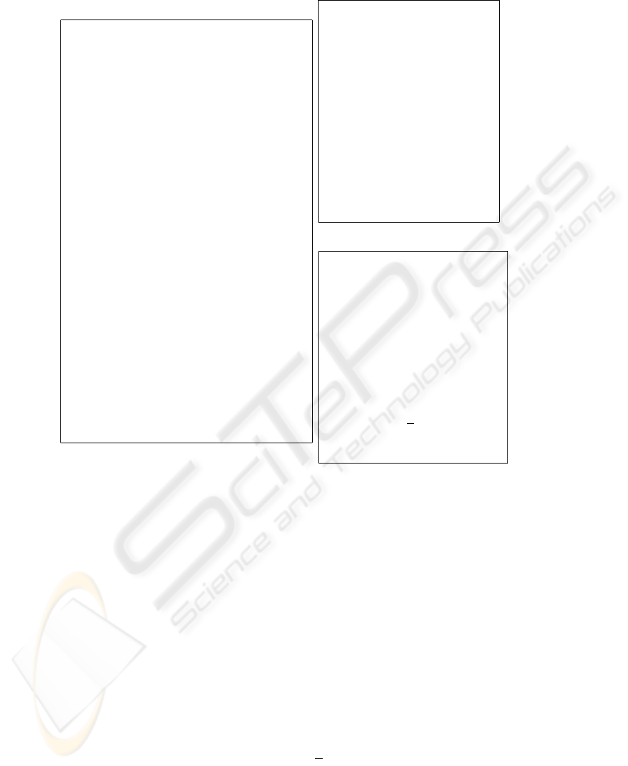
5.1 STAGGER Scenario
The STAGGER concepts scenario is described in detail in [7] and involves a dataset
of 120 instances divided into 3 stages. The target concept changes at an interval of
40 instances. The aim is to track the concept with the highest possible accuracy while
adapting to the changes observed in the data. The experiment was run 100 times and
the average accuracy of the system is shown in Figures 4 (noise free data) and 5 (data
contained 20% noise). The results from using FLORA on the same data are also shown
for comparison purposes. The reason for selecting FLORA is because it uses the most
popular form of tracking drift with a single dynamic window and it implements heuris-
tics routines to adjust the window size based on the changes detected in the data. The
results show that the algorithm presented in this paper tracks the concept with high
59

accuracy and adapts very quickly to the changes in the data. The performance of the al-
gorithm decreases as more noise is added to the data both in terms of tracking accuracy
and speed with which it converges to the target concept. However, when compared with
FLORA, the new algorithm’s performance is better in all three cases and in particular it
adapts faster to the changes in the data.
5.2 Recurrent Concept Scenario
The second experiment used to test the algorithm involved tracking a recurrent concept.
The scenario involved a modified version of the STAGGER concept problem. In this
case we added a fourth stage of 40 instances. The concept from the first 40 instances
was repeated in the third stage of the experiment. The concept from the second stage
was repeated in the fourth stage of the experiment. The success was measured by how
well the system handled the repeated concept. The experiment was run 100 times and
the average accuracy of the system is shown in Figures 6 (noise free data) and 7 (data
contained 20% noise). The results show that the system adapted significantly faster to
the target concept when the concept was repeated. FLORA is also able to recognise past
concepts but its accuracy is slightly lower due to its reliance on instance based concept
generalizations.
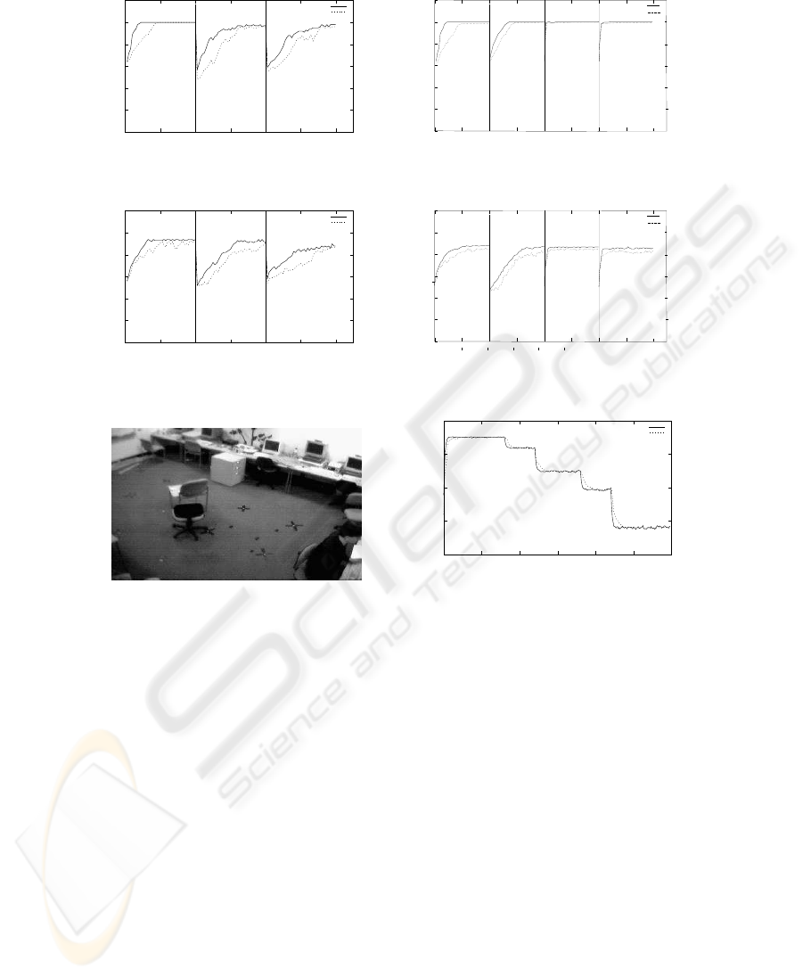
5.3 Background Frame Problem
The third experiment involved tracking changes in the average frame computed from
video surveillance. A simple way to detect motion in surveillance is to analyse the
differences between a preset video frame and the frames obtained from the live sur-
veillance. The problem is that in many cases, gradual changes in the background due
to changes in the environment conditions (such as faulty flashing neon-lights) are in-
terpreted as actual motion which results in a large number of false alarms. The dataset
used for this problem contained 300 video frames from a stationary camera as shown in
Figure 8. The lighting conditions change four times over the 300 frames. The aim for
this problem was to track the changes in the average frame as accurately as possible.
The results are shown in Figure 9. The plot shows the true concept value over the 300
instances as well the concept value derived by the drift tracking algorithm. Overall, the
accuracy of the algorithm is very good and there is little delay before the concept is
adapted to the changes in the data.
6 Conclusions
This paper describes a multiple window algorithm that combines evidence based for-
getting and prediction analysis to track concept drift. The work presented makes two
novel contributions: it introduces a new mechanism for forgetting and it uses a pre-
diction method to control the size of the windows and thus allow a more pro-active
interpretation of the data. The algorithm was tested using two datasets: the STAGGER
concepts problem and a background frame tracking problem. The results obtained show
that the algorithm adapts very quickly to changes in the data and tracks drift with very
good accuracy.
60
0
20
40
60
80
100
120
0 20 40 60 80 100 120
Classification Accuracy
Training Instances Processed
"MRL"
"FLORA"
Fig.4. Classification results of data without
noise.
0
20
40
60
80
100
120
0 20 40 60 80 100 120
Classification Accuracy
Training Instances Processed
"MRL"
"FLORA"
Fig.5. Classification results of data with 20%
noise.
"MRL"
20
40
60
80
100
120
0 20 40 60 80 100 120
Classification Accuracy
140
160
Training Instances Processed
"FLORA"
0
Fig.6. Classification results of data without
noise.
"MRL"
20
40
60
80
100
120
0 20 40 60 80 100 120
Classification Accuracy
140
160
Training Instances Processed
"FLORA"
0
Fig.7. Classification results of data with 20%
noise.
Fig.8. Surveillance Image.
0
0.5
1
1.5
2
0 50 100 150 200 250 300
Luminance Intensity Concept Value
Video Frame Number
"True_Concept_Value"
"MRL_Concept_Value"
Fig.9. Classification results for background
frame problem.
References
1. M. Harries and K. Horn. Learning stable concepts in a changing world. Lecture Notes in
Computer Science, 1359:106–122, 1998.
2. M. Kubat and G. Widmer. Adapting to drift in continuous domains. Lecture Notes in Computer
Science, 912:307–312, 1995.
3. Mihai Lazarescu, Svetha Venkatesh, and Hai Hung Bui. Using multiple windows to track
concept drift. Intelligent Data Analysis, 8(1), 2004.
4. M. Maloof and R. Michalski. Selecting examples for partial memory learning. Machine
Learning, 41:27–52, 2000.
5. M.A. Maloof. Progressive partial memory learning. PhD thesis, School of Information Tech-
nology and Engineering, George Mason University, Fairfax, VA, 1996.
6. M.A. Maloof and R.S. Michalski. AQ-PM: A system for partial memory learning. In Pro-
ceedings of the Eighth Workshop on Intelligent Information Systems, pages 70–79, Warsaw,
Poland, 1999. Polish Academy of Sciences.
61

7. J. Schlimmer and R. Granger. Beyond incremental processing: Tracking concept drift. In
Proceedings of AAAI’86, pages 502–507. AAAI Press, 1986.
8. Gerhard Widmer. Combining robustness and flexibility in learning drifting concepts. In Eu-
ropean Conference on Artificial Intelligence, pages 468–472, 1994.
9. Gerhard Widmer and Miroslav Kubat. Effective learning in dynamic environments by ex-
plicit context tracking. In Machine Learning: ECML-93, European Conference on Machine
Learning, Proceedings, volume 667, pages 227–243. Springer-Verlag, 1993.
62
