MULTIMODELLING STEPS FOR FREE-SURFACE HYDRAULIC
SYSTEMS CONTROL
Eric Duviella, Philippe Charbonnaud and Pascale Chiron
Laboratoire G
´
enie de Production
Ecole Nationale d’Ing
´
enieurs de Tarbes
47, avenue d’Azereix, BP 1629
65016 Tarbes Cedex, France
Keywords:
Multimodelling, operating modes, on-line selection, hydrographic network.
Abstract:
The paper presents multimodelling steps for the design of free-surface hydraulic system control strategies. This
method is proposed to represent simply and accurately the non-linear hydraulic system dynamics under large
operating conditions. It is an interesting alternative to the use of Saint Venant partial differential equations
because it allows the design, the tuning and the validation of control strategies. The multimodelling steps of
the proposed method are performed in order to lead to the determination of a finite number of models. The
models are selected on-line by the minimization of a quadratic criterion. The evaluation of the multimodelling
method is carried out by simulation within the framework of a canal with trapezoidal profile.
1 INTRODUCTION
The hydrographic networks are systems geograph-
ically distributed conveying gravitationally water
quantities. They are composed of open-surface hy-
draulic systems (canals, rivers, etc.) which are used
to satisfy the requests related to human activities. The
efficient management of these systems is essential to-
day, according to the recognized importance of wa-
ter resource. This management requires the proposal,
the design and the tuning of control strategies through
simulation, before their implementation on real sys-
tems. The free-surface hydraulic system dynamics is
characterized by nonlinearity and important transfer
delays. Although the Saint Venant Partial Differen-
tial Equations (PDE) accurately represent hydraulic
systems dynamics (Chow et al., 1988; Malaterre and
Baume, 1998), their resolution involves numerical ap-
proaches according to discretization scheme which
are rather complex to handle in the control strategy
design and tuning steps. The PDE simplification and
linearization around an operating point led to simplify
models of the hydraulic system dynamics (Litrico and
Georges, 1999a). In the literature, most authors have
proposed control strategies based on the PDE lin-
earization (Malaterre et al., 1998). However, the ac-
curacy of these models is only acceptable on restricted
interval around the operating point, and their use on
large operating conditions requires robust controller
design, as proposed in (Litrico and Georges, 1999b).
The representation of the non linear systems with
variable transfer delays involves the identification
problem of a model with variable parameters or mul-
tiple models. In the literature, multimodelling ap-
proaches for the predictive control are described in
(Palma and Magni, 2004) and in (
¨
Ozkan and Kothare,
2005). These methods are based on switching tech-
nics amongst several simple models. In the case of
nonlinear systems with variable transfer delays, an al-
gorithm for estimation of the models most represen-
tative of the system dynamics is proposed in (Petridis
and Kehagias, 1998). In these approaches, the models
number and their operating range are known a priori.
The nonparametric modelling of the nonlinear sys-
tem dynamics can also be carried out by Gaussian ap-
proaches (Gregorcic and Lightbody, 2002). The iden-
tification and control of open-channel systems using
Linear Parameter Varying (LPV) models is proposed
in (Bolea et al., 2004; Puig et al., 2005). The dynam-
ics of hydraulic systems is modelled by a first order
differential equation with time delay. The parameters
of the LPV model have been identified using a pa-
rameter estimation algorithm. These approaches re-
quire an important quantity of adapted data.
In this article, the multimodelling steps which lead
to the determination of a finite number of models, are
proposed to design and tune control strategies for hy-
draulic systems subject to large operating conditions.
32
Duviella E., Charbonnaud P. and Chiron P. (2006).
MULTIMODELLING STEPS FOR FREE-SURFACE HYDRAULIC SYSTEMS CONTROL.
In Proceedings of the Third International Conference on Informatics in Control, Automation and Robotics, pages 32-38
DOI: 10.5220/0001203400320038
Copyright
c
 SciTePress

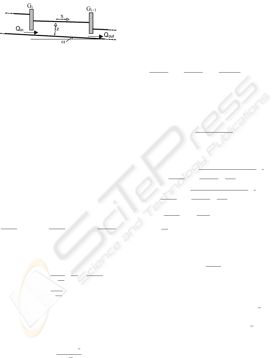
Figure 1: Canal reach.
In section 2, the multimodelling steps according to
the celerity coefficient is described. An on-line mul-
timodels selection method is presented in section 3.
In section 4, the method is used to identify the dy-
namic of a canal with trapezoidal profile. The effec-
tiveness of the multimodelling steps compared to the
Saint Venant PDE is presented in section 5.
2 MODELLING OF
FREE-SURFACE HYDRAULIC
SYSTEMS
Open-channel systems are characterized by large
sized, nonlinear dynamics and important transfer de-
lays. They are generally broken down into several
reaches which are located between two measurement
points or gates G
i
and G
i+1
(see Figure 1). The dif-
fusive wave equation (Chow et al., 1988), expressed
by relation (1) can be used to represent accurately the
canal reach dynamics.
∂Q(x,t)
∂t
+C(Q, z, x)
∂Q(x,t)
∂x
−D(Q, z, x)
∂
2
Q(x,t)
∂x
2
= 0,
(1)
where Q(x, t) is the reach flow discharge [m
3
/s],
C(Q, z, x) the celerity coefficient [m/s] and
D(Q, z, x) the diffusion coefficient [m
2
/s] ex-
pressed by:







C(Q, z, x) =
1
L
2
∂J
∂Q

∂L
∂x
−
∂(LJ)
∂z

,
D(Q, z, x) =
1
L
∂J
∂Q
,
(2)
where L is the water surface width and J is the fric-
tion slope. Several empirical formulas can be used to
express the friction slope J (Kovacs, 1988). Gener-
ally, the Manning-Strickler formula (3) is used. The
friction slope J is considered equal to the canal slope
α when the flow depth is normal:
J =
Q
2
n
2
M
P
4
3
S
10
3
, (3)
where n
M
is the Manning coefficient associated with
the hydraulic system considered (river, channel) and
with his bed type (n
M
lies between 0.02 and 0.01 for
a concrete canal). The Manning coefficient determi-
nation can be carried out from physical knowledge of
the hydraulic system or by identification (Ooi et al.,
2003).
The diffusive wave equation (1) can be lin-
earized around an operating discharge Q
e
(Litrico and
Georges, 1999a), and the identified celerity and diffu-
sion parameters are denoted C
e
and D
e
.
dq(x, t)
dt
+ C
e
dq(x, t)
dx
− D
e
d
2
q(x, t)
dx
2
= 0. (4)
where Q = Q
e
+ q. The discharge variation q from
the reference discharge Q
e
is flowed out with a mean
speed of constant celerity C
e
and is diffused with a
constant diffusion D
e
.
The linearization of the diffusive wave equation
leads to a finite order transfer function:
F (s) =
e
−τ s
1 + a
1
s + a
2
s
2
, (5)
where the transfer function parameters a
1
, a
2
and τ
are calculated by the moment matching method as de-
scribed in (Georges and Litrico, 2002):





























a
1
=
6XD
2
e
C
5
e
+
s
4X
2
D
3
e
C
9
e

9D
e
C
e
− 2X

!
1
3
+
6XD
2
e
C
5
e
−
s
4X
2
D
3
e
C
9
e

9D
e
C
e
− 2X

!
1
3
,
a
2
=
2XD
e
C
3
e

1 −
3D
e
a
1
C
2
e

,
τ =
X
C
e
− a
1
.
The model order is determined according to the
adimensional coefficient C
M
(Malaterre and Baume,
1998):
C
M
=
2C
e
X
9D
e
(6)
where X is the reach length. The canal reach dynamic
is modelled by:
- a second order plus delay transfer function (5) when
C
M
> 1,
- a first order plus delay transfer function when
4
9
<
C
M
≤ 1, with a
2
= 0,
-a first order transfer function when C
M
≤
4
9
, with
a
2
= 0 and τ = 0.
The linearization of the diffusive wave model leads
to the identification of dynamics of free-surface hy-
draulic systems. Validity of the model decreases as
the operating point of system moves away from the
identification point. Accurate representation of open-
surface hydraulic system dynamic on large operating
MULTIMODELLING STEPS FOR FREE-SURFACE HYDRAULIC SYSTEMS CONTROL
33

conditions requires a multimodelling method. It in-
volves to determine the necessary number of models,
i.e. Operating Modes (OM), and their validity bound-
aries.
3 MULTIMODELLING STEPS OF
FREE-SURFACE HYDRAULIC
SYSTEMS
The multimodelling method consists in defining the
models number n necessary to represent the sys-
tem dynamics under large operating conditions. The
process model M of the hydraulic system is de-
composed into a finite class of linear models M =
{M
1
, M
2
, .....M
n
}, where the i
th
linear model of the
hydraulic system is denoted M
i
, and n = card(M ).
The celerity coefficient values are used in order to fix
the number n of OM.
The open-surface hydraulic system dynamics un-
der large operating conditions are represented by the
following relation:

˙x = A
i
x(t) + B
i
u(t − τ),
y = C
i
x(t),
(7)
where u and y are respectively the input and output
variables, x the state. Identification matrices A
i
, B
i
and C
i
are computed for the model M
i
which cor-
responds to the i
th
OM. They are expressed, accord-
ing to the transfer functions (5), by relation: A
i
=

−
a
1i
a
2i
1
−
1
a
2i
0

, B
i
=

0
1
a
2i

and C
i
= [
1 0
].
The celerity coefficient can be considered as the
most representative parameters of the open-channel
system dynamics. Therefore, a model is considered
as available as soon as the error on the celerity coef-
ficient is inferior to a fixed percentage Π
c
. The valid-
ity boundaries are defined for each OM. The value of
parameter Π
c
is choosen according to the system dy-
namics. The multimodelling method is described by
an algorithm (see Table 1), where the OM are deter-
mined starting with C
med
. This one is computed with
the parameters C
min
and C
max
corresponding respec-
tively to the minimum and maximum discharges of
the system Q
min
and Q
max
.
This algorithm leads to the determination of the
celerity coefficient C
id
r
used to identify the r
th
lin-
ear model and the OM validity boundaries C
inf
r
and
C
sup
r
. According to C
id
r
, the water elevation z
id
r
of each r
th
OM are determined, with one millimeter
accuracy, by the digital resolution of the relation (8)
with Newton method.
C
id
=
√
JS
5
3
nP
2
3
L
2

−
1
2
∂L
∂z
−
L
3P

2
∂P
∂z
− 5
P
S
∂S
∂z

,
(8)
Table 1: Multimodelling Algorithm.
Input : C
max
, C
min
, Π
C
Output : C
id
r
, C
sup
r
, C
inf
r
,
C
med
=
C
max
+ C
min
2
,
r = 1,
For i :






ln
C
min
C
med
ln
(1 + Π
C
)
(1 − Π
C
)






to






ln
C
max
C
med
ln
(1 + Π
C
)
(1 − Π
C
)






,















C
id
r
=

1 + Π
C
1 − Π
C

i
C
med
,
C
sup
r
= (1 + Π
C
)

1 + Π
C
1 − Π
C

i
C
med
,
C
inf
r
= (1 − Π
C
)

1 + Π
C
1 − Π
C

i
C
med
,
r + +,
EndFor.
where L, P and S parameters are expressed, accord-
ing to the geometrical characteristics, interms of the
water elevation z
id
. The computation of water eleva-
tion z
id
r
allows for the determination of the diffusion
coefficient D
id
r
(2). Finally, the matrices A
i
, B
i
and
C
i
are computed using C
id
r
and D
id
r
values.
The multimodelling method is used to identify the
free-surface hydraulic system dynamics with several
OM. The discharge boundary conditions Q
inf
i
and
Q
sup
i
are computed according to the relation:
Q =
√
JS
5
3
n
M
P
2
3
, (9)
where P and S parameters depend on the water ele-
vation boundary conditions z
inf
r
and z
sup
r
.
The presented algorithm can be used for various
hydraulic system profiles, i.e. rectangular, trapezoidal
and circular profiles. The multimodelling steps were
used in (Duviella et al., 2006) within the framework
of a dam gallery with a circular profile. In order
to simulate and implement control strategies for hy-
draulic systems under large operating conditions, it is
necessary to propose an on-line selection method of
the multi model.
ICINCO 2006 - SIGNAL PROCESSING, SYSTEMS MODELING AND CONTROL
34

4 ON-LINE SELECTION
CRITERION OF OPERATING
MODE
An analytical expression of the hydraulic system out-
put y can be approached as:
y ' ˆy =
n
X
j=1
δ
j
m
.y
j
, (10)
where n is the number of OM, m denotes the actual
OM, y
j
is the answer of the j
th
model M
j
, and δ
j
m
is
equal to 1 if m = j and 0 otherwise. The main prob-
lem of OM detection lies in the real-time estimation
of m at the boundary between two OM, i.e., the cur-
rent behavior of the physical process. The selection
method has to figure out the OM actual value. For
that, a criterion J
j
(11), 0 < j ≤ n, is defined for
each OM and computed at each sample period kT
s
.
J
j
(k) =
1
N − 1
N−1
X
i=0
ε
j,i
(k), (11)
where N is the size of a sliding window, ε
j,i
(k) is the
j
th
identification error and:
ε
j,i
(k) = (y(k − i) − y
j
(k − i))
2
. (12)
The multi-model output recursive square error cri-
terion J(k) = [J
1
(k) J
2
(k) ... J
j
(k)...] is computed
with the recursive formula:
J
j
(k) = J
j
(k −1) +
1
N − 1
(ε
j,0
(k) −ε
j,0
(k −N)).
(13)
At each sampling period, a minimization of the cri-
terion given by (11) is carried out to determine the ad-
equat transfer function. The correspondant OM num-
ber is denoted d(k) and satisfies:
d(k) = arg min
1≤j≤n
J
j
(k)}. (14)
At the starting time, it is assumed that d(0) = 1.
The detection time is defined by:
t
d
(k) = {kT
s
, d(k) 6= d(k − 1)}, (15)
The multimodelling steps which lead to determine
the different OM, associated to on-line selection cri-
terion, makes possible to represent the hydraulic sys-
tems dynamics on the totality of their operating range.
In the following section, the multimodelling steps
and on-line selection criterion are illustrated within
the framework of a canal with trapezoidal profile.
The multimodelling approach is then compared to a
method based on Saint Venant equations.
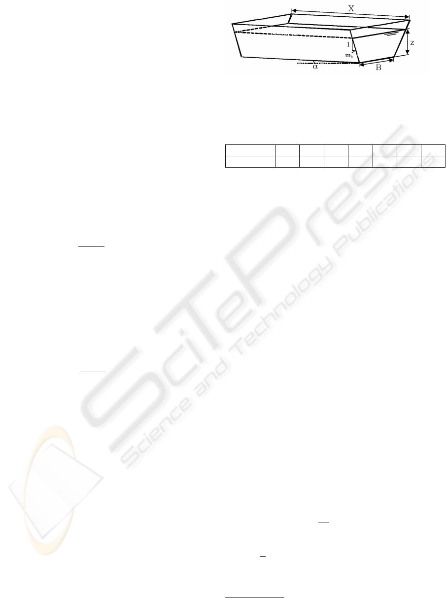
Figure 2: Canal reach with trapezoidal profile.
Table 2: Canal reach downstream limiting conditions.
Q [m
3
/s] 0.5 1.4 2.6 4.2 6.2 8.7 10
z [m] 0.3 0.5 0.7 0.9 1.1 1.3 1.4
5 APPLICATION TO A CANAL
WITH TRAPEZOIDAL
PROFILE
The application of the multimodelling steps is carried
out on a canal reach with a trapezoidal profile (see
Figure 2). Its geometrical characteristics are given be-
low:
- bottom width B = 2.85 m,
- average fruit of the banks m
b
= 0.99,
- profile length X = 1732 m,
- Manning coefficient n
M
= 0.02,
- reach slope α = 0.13 %,
- minimal discharge Q
min
= 1 m
3
/s,
- maximal discharge Q
max
= 10 m
3
/s.
This canal reach is firstly modelled by the Saint
Venant equations, and secondly by the multimod-
elling approach. The resolution of Saint Venant equa-
tions is realized with the downstream limiting con-
ditions (see Table 2) according to the software SIC
1
.
This one allows the dynamic simulation of rivers and
canals according to the Preissmann scheme. Among
the resolution algorithms proposed, the Newton algo-
rithm which offers the best performances in spite of a
longer simulation time, is chosen. To avoid the insta-
bility periods during simulation, the time and space
steps must be tuned so that the Courant number (16)
is equal to one.
Cr =
dt
dx
(V + C), (16)
where V is the mean velocity of the flow expressed
by V =
Q
S
.
The multimodelling step applied according to the
algorithm (see Table 1) with an tolerated error Π
c
of
10% leads to the identification of three OM. In the
1
SIC user’s guide and theorical concepts. CEMAGREF,
Montpellier, 1992. http://canari.montpellier.cemagref.fr/
MULTIMODELLING STEPS FOR FREE-SURFACE HYDRAULIC SYSTEMS CONTROL
35

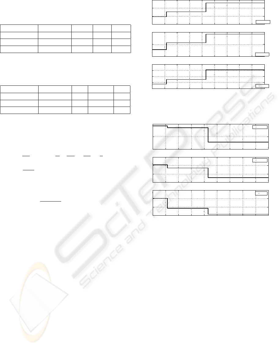
Table 3: Identification discharge Q
id
r
, operating range Ω
r
,
and characteristics z
id
r
, C
id
r
and D
id
r
of each OM.
Q
id
r
[m
3
/s] Ω
r
[m
3
/s] z
id
r
C
id
r
D
id
r
1.5 [1 ; 2.2[ 0.469 1.3 148
3.4 [2.2 ; 5.3[ 0.775 1.6 300
8.7 [5.3 ; 10] 1.320 1.9 617
Table 4: Identification discharge Q
id
r
, operating range Ω
r
,
and characteristics a
1i
, a
2i
and τ
i
of each OM.
Q
id
r
[m
3
/s] Ω
r
[m
3
/s] a
1i
a
2i
τ
i
1.5 [1 ; 2.2[ 742 154520 608
3.4 [2.2 ; 5.3[ 736 135470 369
8.7 [5.3 ; 10] 678 77690 226
case of a hydraulic system with a trapezoidal profile,
celerity C
e
and diffusion D
e
are expressed by:
C
e
=
Q
e
L
2

−m
b
+
L
3

2B
P z
+
5L
S
−
2
z

,
D
e
=
Q
e
2LJ
,
(17)
with :
- L = B + 2m
b
z,
- S = (B + m
b
z)z,
- P = B + 2z
√
1 + m
b
2
.
The three OM, the correspondant identification dis-
charge Q
id
r
, operating range Ω
r
, and characteristics
z
id
r
, C
id
r
and D
id
r
are given in Table 3. Characteris-
tics a
1i
, a
2i
and τ
i
are given in Table 4.
In order to visualize the identified OM, parameters
z
id
r
, C
id
r
and D
id
r
are represented in Figure 3, and
parameters a
1
, a
2
and τ in Figure 4 according to the
discharge Q. The values of each parameter were cal-
culated beforehand for each discharge of the operat-
ing range, i.e. [1; 10], with a step of 1 m
3
/s. These
values are represented by points in Figures 3 and 4.
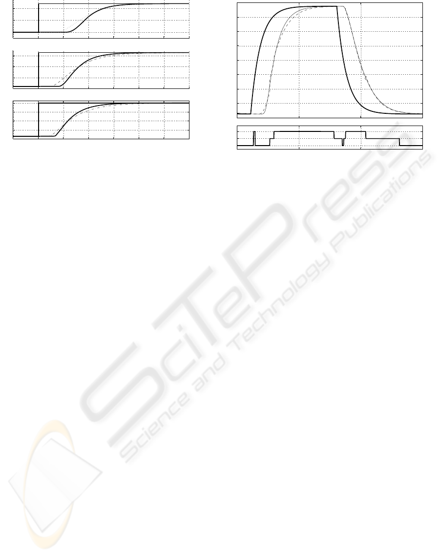
The evaluation of the multimodelling approach is
carried out by comparison with the Saint Venant ap-
proach. Figure 5 shows the responses to steps around
the discharges used for the parameters identification
of the three OM. The setpoints are in bold continuous
line, the outputs resulting from SIC are also in bold
continuous line, those resulting from the first model
M
1
are in dot line, those resulting from the second
M
2
are in dashed line, and finally those resulting from
the third M
3
are in dash-dot line.
Figure 5.a shows the M
1
and Saint Venant answers
of a step of 1.2 m
3
/s starting from a discharge of 1
m
3
/s, Figure 5.b, the answers of a step of 3.1 m
3
/s
starting from a discharge of 2.2 m
3
/s, and Figure 5.c,
the answers of a step of 3.7 m
3
/s starting from a dis-
0
0.5
1
1.5
(a)
C [m/s]
1
1.5
2
(b)
Z [mm]
1 2 3 4 5 6 7 8 9 10
0
200
400
600
800
(c)
D [m
2
/s]
C(q)
z(q)
z( Q)
C(Q)
D(q)
q [m
3
/s]
Figure 3: Variation of the parameters z, C and D according
to the considered OM.
650
700
750
(a)
a
1
0.5
1
1.5
2
x 10
5
(b)
a
2
1 2 3 4 5 6 7 8 9 10
200
400
600
800
(c)
τ
(q)
a2(q)
a1(q)
q [m
3
/s]
τ
[s]
Figure 4: Variation of the parameters a
1
, a
2
and τ accord-
ing to the considered OM.
charge of 5.3 m
3
/s. According to the simulation re-
sults, the dynamics modelled by transfer functions are
close to those from SIC for each OM.
Then, the comparison between the two modelling
approaches is carried out by simulation on the whole
operating range of the canal reach. The setpoint input
is represented in bold continuous line in Figure 6.a.
It corresponds to setpoints with discharge amplitude
from 1 to 9 m
3
/s.
The simulation results obtained by SIC are repre-
sented in continuous line, and those from multimod-
elling in dashed line in Figure 6.a. The on-line selec-
tion of the transfer function is represented in Figure
6.b. This selection is realized according to the rules
presented in section 4.
The outputs resulting from the two approaches are
very similar on the totality of the canal reach oper-
ating range. Light differences between these outputs
appear around 8 m
3
/s when the discharge increase.
ICINCO 2006 - SIGNAL PROCESSING, SYSTEMS MODELING AND CONTROL
36

1
1.5
2
(a)
Q [m
3
/s]
2
3
4
5
(b)
Q [m
3
/s]
0 10 20 30 40 50 60 70
5
6
7
8
9
(c)
Time [min]
Q [m
3
/s]
Figure 5: Input step setpoints (bold continuous line) ar-
round (a) 1.5 m
3
/s, (b) 3.5 m
3
/s and (c) 8.5 m
3
/s, and
corresponding outputs resulting from SIC (bold continuous
line), from M
1
(dot line), M
2
(dashed line) and M
3
(dash-
dot line).
The maximum output error between these two ap-
proaches is reached for 7.5 m
3
/s and corresponds
to an error percentage of 4.2 %. These differences
are sufficiently weak to conclude on the effective-
ness of the multimodelling approach. Moreover for
this simulation case, the excecution time for the SIC
method was ten times longer than for the multimod-
elling method.
The multimodelling approach interest lies in the
faithful representation of the hydraulic systems dy-
namics on the totality of their operation range, and
in the facility of its implementation. This approach
requires only the knowledge of the physical charac-
teristics of the hydraulic system, the OM determi-
nation and the on-line selection method implementa-
tion. Moreover, the multimodelling approach consti-
tutes an effective tool for the design and the tuning of
regulation and reactive control strategies.
6 CONCLUSION
The efficient management of hydraulic systems re-
quired the proposal and the design of regulation and
reactive control strategies. The development of these
techniques is facilitated using an operational and
faithful simulation tool. A multimodelling approach
is proposed to design and tune the control strategies
of hydraulic systems subject to large operating condi-
tions. It leads to obtain a finite number of operating
modes accurately reproducing the hydraulic systems
dynamics around operating discharges. This multi-
modelling method is carried out by considering an
acceptable percentage of error on the celerity. The
on-line operating modes selection method based on
1
2
3
4
5
6
7
8
9
(a)
Q [m
3
/s]
0 1 2 3
F1
F2
F3
(b)
M
i
(s) Selection
Time [h]
Figure 6: (a) Setpoint input (bold continuous line), SIC
output (continuous line) and multimodelling output (dashed
line) and (b) β the selected transfer function.
the minimization of a quadratic criterion leads to the
accurate identification of the adequat model.
The multimodelling steps and the on-line operat-
ing modes selection criterion are illustrated within the
framework of a canal reach with trapezoidal profile.
The dynamic identified by multimodel are compared
to those resulting from a discretization scheme us-
ing for the Saint Venant equations resolution. Simu-
lation results lead to conclude to the multimodelling
approach effectiveness.
REFERENCES
Bolea, Y., Puig, V., Blesa, J., Gomez, M., and Rodellar, J.
(2004). An LPV model for canal control. 10th IEEE
International Conf
´
erence on Methods and Models in
Automation and Robotics, MMAR, 30 August - 2 Sep-
tember, Miedzyzdroje, Poland, 1:659–664.
Chow, V. T., Maidme nt, D. R., and Mays, L. W. (1988).
Applied Hydrology. McGraw-Hill, New York, Paris.
Duviella, E., Chiron, P., and Charbonnaud, P. (2006). Mul-
timod
´
elisation des syst
`
emes hydrauliques
`
a surface li-
bre. Conf
´
erence Francophone de Mod
´
elisation et Sim-
ulation, MOSIM’06, Rabat (Maroc), 3-5 avril.
Georges, D. and Litrico, X., editors (2002). Automatique
Pour la Gestion Des Ressources En Eau. Herm
`
es Sci-
ence Publications, Lavoisier, 11 rue Lavoisier, 75008
Paris.
Gregorcic, G. and Lightbody, G. (2002). Gaussian
processes for modelling of dynamic non-linear sys-
tems. In Proc. of the Irish Signals and Systems Con-
ference, ISSC’02, Cork, Ireland, 25-26 Juin 2002.
Kovacs, Y. (1988). Mod
`
eles de Simulation D’
´
ecoulement
Transitoire En Reseau D’assainissement. PhD thesis,
ENPC - CERGRENE.
MULTIMODELLING STEPS FOR FREE-SURFACE HYDRAULIC SYSTEMS CONTROL
37

Litrico, X. and Georges, D. (1999a). Robust continuous-
time and discrete-time flow control of a dam-river sys-
tem. (i) modelling. Applied Mathematical Modelling
23, pages 809–827.
Litrico, X. and Georges, D. (1999b). Robust continuous-
time and discrete-time flow control of a dam-river
system. (II) controller design. Applied Mathematical
Modelling 23, pages 829–846.
Malaterre, P., Rogers, D., and Schuurmans, J. (1998). Clas-
sification of canal control algorithms. Journal of irri-
gation and drainage engineering, 124(1):3–10.
Malaterre, P.-O. and Baume, J.-P. (1998). Modeling and
regulation of irrigation canals: Existing applications
and ongoing researches. IEEE International Con-
ference on Systems, Man, and Cybernetics, 4:3850–
3855.
Ooi, S. K., Krutzen, M., and Weyer, E. (2003). On phys-
ical and data driven modelling of irrigation channels.
Control Engineering Practice, 13:461–471.
¨
Ozkan, L. and Kothare, M. V. (2005). Stability analysis of
a multi-model predictive control algorithm with ap-
plication to control of chemical reactors. Journal of
Process Control, In Press, Corrected Proof.
Palma, F. D. and Magni, L. (2004). A multi-model struc-
ture for model predictive control. Annual Reviews in
Control, , Issue 1, 28:Pages 47–52.
Petridis, V. and Kehagias, A. (1998). A multi-model algo-
rithm for parameters estimation of time-varying non-
linear systems. Automatica, Elsevier Science Ltd,
34(4):469–475.
Puig, V., Quevedo, J., Escobet, T., Ch arbonnaud, P., and
Duviella, E. (2005). Identification and control of an
open-flow canal using LPV models. CDC-ECC’05,
44 th IEEE conference on decision and control and
european control conference, Seville, Spain, 12-15 de-
cember 2005, pages 1893–1898.
ICINCO 2006 - SIGNAL PROCESSING, SYSTEMS MODELING AND CONTROL
38