INTERACTION CONTROL EXPERIMENTS FOR A ROBOT WITH
ONE FLEXIBLE LINK
L. F. Baptista
Escola N
´
autica Infante D. Henrique
Av. Engenheiro Bonneville Franco, 2770-058 Paco de Arcos
J. M. M. Martins, J. M. G. S
´
a da Costa
Instituto Superior T
´
ecnico, GCAR/IDMEC
Av. Rovisco Pais, 1049-001 Lisboa Codex
Keywords:
Flexible-link manipulator, closed-loop inverse kinematics, interaction control, real-time control.
Abstract:
One of the major drawbacks of flexible-link robot applications is its low tip precision, which is an essential
characteristic for applications with interaction control with a contact surface. In this work, interaction control
strategies considering rigid and flexible contact surfaces are applied on a two degrees of mobility flexible-link
manipulator. The interaction strategies are based on the closed-loop inverse kinematics algorithm (CLIK) to
obtain the angular references to the joint position controller. The control schemes were previously tested by
simulation and further implemented on the flexible-link robot. The obtained experimental results exhibit a
good force tracking performance, especially for a rigid surface, and reveal the successful implementation of
these control architectures for a robot with one flexible link.
1 INTRODUCTION
The evolution of industrial manufacturing, lead to the
necessity of optimize the production, where the main
goal is to achieve best quality products at lower prices.
The manipulator robot is a crucial automation equip-
ment that fulfill these requirements, due to its high
productivity and easy adaptation to a large number of
complex and repetitive tasks. The manipulator robots
have also the ability to work in adverse environments
to the human workers. Due to these characteristics,
the study of robot manipulator control has received a
growing attention by a lot of researchers during the
last decades, in order to design robots with high per-
formance (Canudas de Wit et al., 1998).
In general, industrial robots have rigid mechanical el-
ements which leads to a high power consumption. To
overcome this disadvantage, lightweight and flexible
links have been considered in the construction of new
robots. These new links allow the same mobility ca-
pacity as the rigid robots with a lower power con-
sumption. Also, due to the lighter weight of the links,
the interaction with the environment, especially in the
case of collision, cause less damage.
When a manipulator robot executes an interaction
task, the tip or end-effector enters in contact with the
environment and a certain force is exerted on the sur-
face. Since it’s necessary to achieve an high preci-
sion tip position to obtain a good interaction force
control, advanced control algorithms have been de-
veloped to obtain a high force tracking performance
(Zeng and Hemami, 1997). However, flexible-link
manipulators exhibit an important drawback in com-
parison with rigid robots, due to the difficulty in con-
trol its tip or end-point position. The flexibility rises
the dynamic coupling, the non-linearities, and gives
to the robot infinite degrees of freedom derived from
the vibration modes of the flexible elements. Due to
these vibrations, the system becomes a non-minimum
phase system (Talebi et al., 1998). The zeros in the
right semi-plan, due to the non minimum phase lead
to an unstable system, when the tip position is directly
controlled through feedback.
To avoid these drawbacks, several techniques to ef-
ficiently control flexible-link robots have been stud-
ied. The control of a flexible manipulator at the joint
level has been established by a lot of authors like
(Khorrami and Jain, 1994) for the tracking problem
and (Vandegrift et al., 1994) for the regulation prob-
lem, among others. One of the proposed strategies
to solve the inverse kinematics problem for flexible
arms, was derived from the closed loop inverse kine-
matics algorithm (CLIK) developed for rigid manip-
ulators (Siciliano, 1990). The inverse kinematics for-
mulation with feedback of joint coordinates and de-
flection variables for constrained flexible manipula-
66
F. Baptista L., M. M. Martins J. and M. G. Sá da Costa J. (2006).
INTERACTION CONTROL EXPERIMENTS FOR A ROBOT WITH ONE FLEXIBLE LINK.
In Proceedings of the Third International Conference on Informatics in Control, Automation and Robotics, pages 66-73
DOI: 10.5220/0001204900660073
Copyright
c
 SciTePress

tors was developed by (Siciliano, 1999; Siciliano and
Villani, 2001). Finally, more complex algorithms for
solving the inverse kinematics problem at high speed
velocities with flexible manipulators have been pro-
posed by (Cheong et al., 2004).
The purpose of this work is to obtain experimental re-
sults with interaction control algorithms for a planar
robot with two revolute joints and two links, where
the second link is flexible. The control strategies were
implemented considering the CLIK algorithm to ob-
tain the desired angular references to the joint position
controller. The interaction control algorithm was ap-
plied considering rigid and flexible contact surfaces,
respectively.
The outline of the paper is as follows. Section 2 de-
scribes the flexible link forward and inverse kinemat-
ics formalism and the closed loop inverse kinematics
algorithm (CLIK). In section 3 a brief overview of the
CLIK-based interaction controllers for rigid and flex-
ible surfaces are described. Section 4 describes the
planar flexible-robot setup, the hardware and software
control architecture considered for the real-time ex-
periments. In section 5 the obtained interaction con-
trol results in real-time are presented. Finally, in sec-
tion 6 some conclusions are drawn.
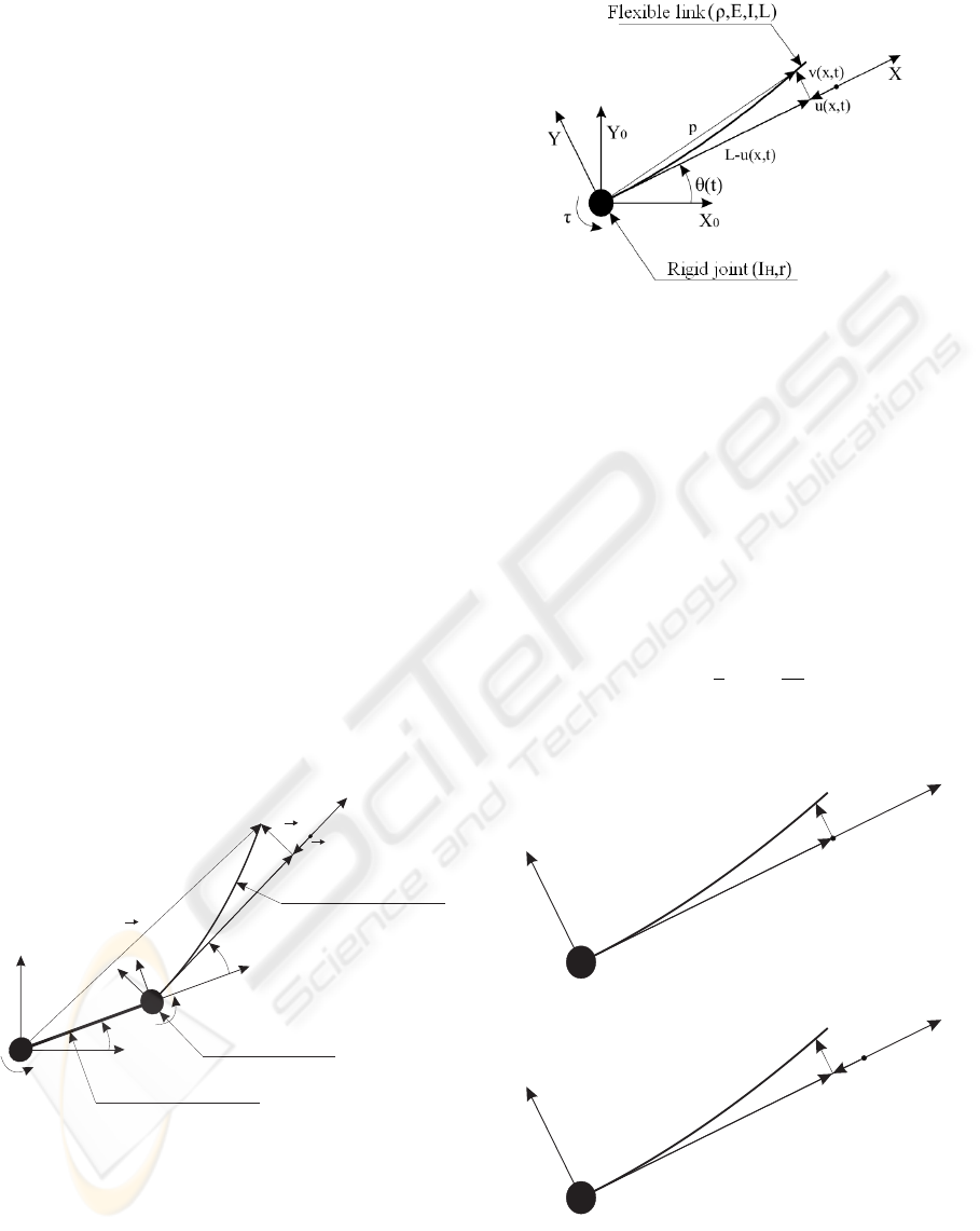
2 FLEXIBLE LINK KINEMATICS
Let us consider a planar robot with two degree of mo-
bility, where the first link is rigid and the second link
is flexible, as depicted in fig. 1.
τ1
Rigidjoint(m ,I ,r)H H
Flexiblelink( ,L)ρ,E,I
2
X0
Y0
τ2
X1
Y2
X2
Y1
θ2
θ1
Rigidlink(m I L)R R, ,
1
u
v
L-u
p
Figure 1: Planar flexible robot schematics.
The robot’s flexible link can be modeled as an
Euler-Bernoulli cantilever, with length L. The flex-
ible link is attached to a rigid joint. When a torque τ
is applied to the rigid joint, the flexible link is rotated
by an angle θ between the body frame {X,Y ,Z} and
the base reference frame {X
0
,Y
0
,Z
0
}, as illustrated in
fig. 2.
Figure 2: Flexible link scheme deflection caused by an ap-
plied torque.
In this figure, v(x, t), represents the lateral dis-
placement point x along the flexible link, relative to
X axis. Thus, the projection of x on X axis will
be given by L − u(x, t) coordinate. Two models
are considered to obtain the length reduction coordi-
nate u(x, t): linear and quadratic models. The lin-
ear model approach considers that length reduction is
null, i.e. u(x, t) = 0. In the quadratic model ap-
proach, length reduction is calculated by the follow-
ing expression
u(x, t) = −
1
2
Z
x
r

dv
dξ

2
dξ (1)
In fig. 3 both length reduction approach due to an elas-
tic link deflection are represented.
X
Y
v(x,t)
L
(a) Linear model
X
Y
u(x,t)
v(x,t)
L-u(x,t)
(b) Quadratic model
Figure 3: Elastic link length reduction models.
In the following, the Assumed Modes discretizing
INTERACTION CONTROL EXPERIMENTS FOR A ROBOT WITH ONE FLEXIBLE LINK
67

method (Martins, 2000) will be considered for the lat-
eral displacement v calculation. This method consider
v(x, t) = χ(x)δ(t) (2)
where χ are the normalized mode shapes and δ are the
generalized elastic coordinates. Considering only the
two first vibration modes, v is given by
v(x, t) =
2
X
k=1
χ
i
(x) δ
i
(t) (3)
For this particular flexible-link robot, χ
i
are given by
(Nabais, 2002):
χ
1
= 3

x
L

2
− 2

x
L

3
χ
2
= −

x
L

2
+

x
L

3
(4)
where x as referred above, is a point on the elastic
link. Vector ~p represented in fig. 1 is the position on
the link relative to reference frame {X
0
,Y
0
,Z
0
}. This
vector is represented by
~p = ~p
1
+ R
2
0
( ~p
2
− ~u + ~v) (5)
where R
2
0
represents the rotation matrix and ~p
1
is the
position on the first link relative to reference frame
{X
0
,Y
0
,Z
0
}. Also, ~p
2
is the non-deformed second
link end-effector position relative to reference frame
{X
2
,Y
2
,Z
2
}. Summing ~p
2
, ~u and ~v, leads to:
~p = ~p
2
− ~u + ~v (6)
The rotation matrix R
2
0
that describes the position p
relative to reference frame {X
0
,Y
0
,Z
0
} is represented
by:
R
2
0
=

cos(θ
1
+ θ
2
) −sin(θ
1
+ θ
2
)
sin(θ
1
+ θ
2
) cos(θ
1
+ θ
2
)

(7)
Considering that p is the end-effector or tip position,
~p represents the forward kinematics of the flexible-
link robot. Thus, the forward kinematic equations are
given by:

p
x
p
y

=

L
1
cos(θ
1
)
L
1
sin(θ
1
)

+R
2
0

L
2
− ||~u||
||~v||

(8)
which leads to the following equations:
p
x
= L
1
cos(θ
1
) + (L
2
− ||~u||) cos(θ
1
+ θ
2
)
−||~v|| sin(θ
1
+ θ
2
) (9)
p
y
= L
1
sin(θ
1
) + (L
2
− ||~u||) sin(θ
1
+ θ
2
)
+||~v|| cos(θ
1
+ θ
2
)
where ||~u|| and ||~v|| are given by eq. (1) and eq. (3),
respectively.
The inverse kinematics equations relate the cartesian
position coordinates, given by eq. (9), and the joint θ
and deflection δ coordinates. Replacing the equations
(1)-(3) into (9), two equations and four unknown vari-
ables (θ
1
, θ
2
, δ
1
, δ
2
) are obtained. Thus, the system is
undetermined and other methods should be exploited
to overcome this problem.
2.1 CLIK Algorithm
To solve the problem presented above, the Closed
Loop Inverse Kinematics algorithm (CLIK) devel-
oped for rigid robots was adopted in this work, ac-
cording to (Siciliano, 1999). This algorithm feeds
back the joint angles θ calculated by the CLIK al-
gorithm in a closed loop dynamic system in order to
obtain the reference values to the joint position con-
troller. This algorithm is given by (Siciliano and Vil-
lani, 2001):
˙
θ
d
= J
T
p
(θ)K
P
(p
d
− p ) (10)
where:
•
˙
θ
d
are the desired joint velocities,
• J
p
= J
θ
i.e., the rigid part of the Jacobian matrix,
• p
d
is the desired tip position,
• p is the cartesian position determined by forward
kinematics with coordinates θ,
• K
P
is a proportional gain matrix
To obtain the joint references θ
d
for real-time control,
it is necessary to integrate the joint velocities given by
eq. (10). Thus, the discrete version of θ
d
, is given by:
θ
d
(t
k+1
) = θ
d
(t
k
)+T
s
J
T
p
(θ
d
(t
k
))K
P
(p
d
(t
k
)−p(t
k
))
(11)
where
• θ
d
are the reference joint angles for the position
controller,
• T
s
is the sampling period
3 INTERACTION CONTROL
3.1 Rigid Surface
Let us consider that the robot is in contact with a rigid
surface. The restriction imposed by the surface, is
described by
φ(p) = φ(k(θ, δ)) = 0 (12)
Assuming that the robot is in a static condition, the
deflections satisfy the following equation:
Kδ = −J
T
δ
(θ, δ)λj
φ
(13)
where K is the robot stiffness matrix, j
φ
is the equa-
tion gradient (12), defined by
j
φ
=

∂φ
∂p

T
(14)
and λ is the Lagrange multiplier associated with the
restriction. From eq. (13), δ is given by
δ = −K
−1
f (15)
ICINCO 2006 - ROBOTICS AND AUTOMATION
68

where,
f = J
T
δ
(θ, δ)λj
φ
(16)
Differentiating (15) leads to
˙
δ = −K
−1
J
f
(θ, δ)
˙
θ (17)
where
J
f
=
∂f
∂θ
= λj
φ
∂J
T
δ
(θ, δ)
∂θ
(18)
and,
˙
θ = J
T
p
(θ, δ)K
P
(p
d
− p ) (19)
The Jacobian J
p
is defined by
J
p
= J
θ
(θ, δ) − J
δ
(θ, δ)K
−1
J
f
(θ, δ) (20)
where e
p
is the difference between the desired tip po-
sition and the cartesian position determined by the ro-
bot forward kinematics. The joint angles and the de-
flection coordinates are given by the CLIK algorithm.
Discretizing these coordinates, leads to
θ
d
(t
k+1
) = θ
d
(t
k
) + T
s
J
T
p
(θ
d
(t
k
), δ
d
(t
k
))K
P
e
p
(t
k
)
(21)
and
δ
d
(t
k+1
) = −K
−1
(J
T
δ
(θ
d
(t
k
), δ
d
(t
k
))λ(t
k
)j
φ
(22)
Notice that the Jacobian J
p
not only depends on θ co-
ordinates, but also depends on δ coordinates. This
happens because δ depends on f
d
, i.e. the force that
should be applied by the robot on the surface.
The overall interaction controller applies a joint po-
sition PD controller plus the desired force f
d
. The
control law is described by
τ = K
p
(θ
d
− θ) − K
d
˙
θ + J
T
θ
(θ, δ)f
d
n (23)
where n is the normal to the surface and f
d
is the de-
sired force. Notice that the PD controller doesn’t con-
trol directly the interaction force between the tip of
the link and the contact surface. In fact, only the joint
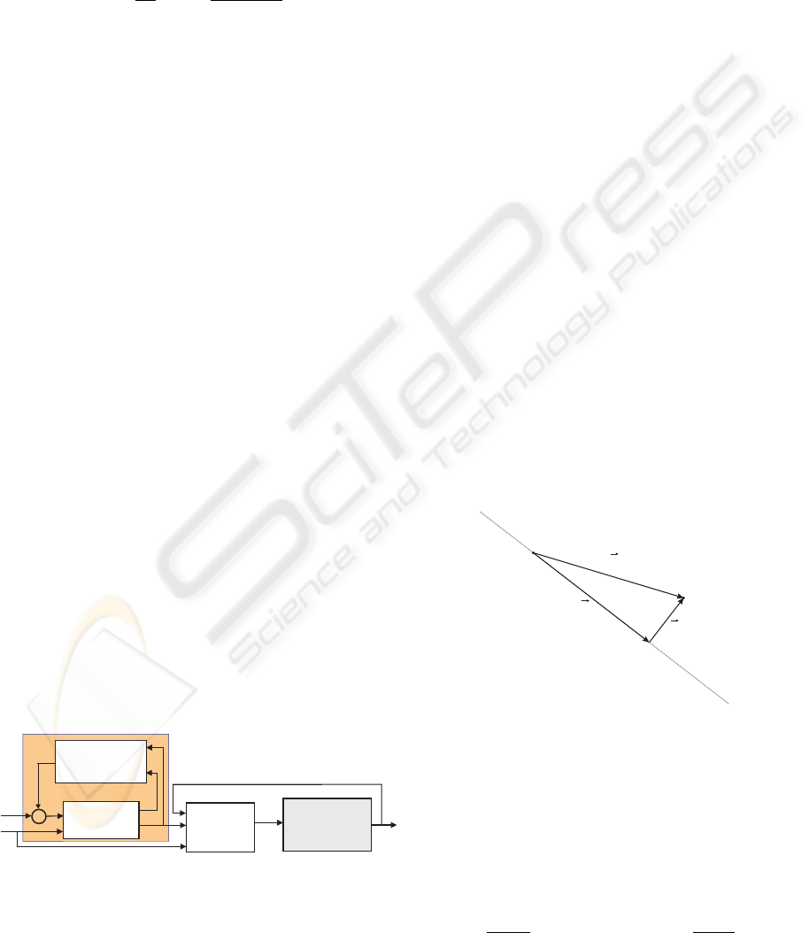
angles are controlled. In fig. 4 the simplified block di-
agram of the CLIK-based interaction controller con-
sidering a rigid surface is represented.
Jointposition
controller
Forwardkinematics
(Flexiblelink)
CLIK
algorithm
Flexible-link
robot
InverseKinematicsStructure
-
+
t
q
q
d
e
p
p
d
d
f
d
p
d
Figure 4: Simplified block diagram of the CLIK-based in-
teraction controller for a rigid surface.
3.2 Flexible Surface
In this case, the interaction control algorithm is sim-
ilar to the previous presented algorithm for the rigid
surface. The main difference concerns with the calcu-
lation method of the reference force, which is based
on the estimated stiffness surface coefficient k
e
. No-
tice that, for simplicity, the environment is modeled as
a linear spring. Due to this assumption, the deflection
coordinates δ, the Jacobian J
p
and the trajectory plan-
ning algorithm will be slightly different (Siciliano and
Villani, 2001).
In the interaction control algorithm considering a
rigid surface described above, the contact force is rep-
resented by the Lagrange multiplier λ. In this case,
the force is represented by
f
d
= k
e
~p
f
(24)
In the interaction controller with a flexible surface,
the desired trajectory has two components, one tan-
gent to the contact surface ~p
s
and another component
normal to the surface ~p
f
. With these two components,
the desired reference trajectory is represented by the
following equation
~p
d
= ~p
s
+ ~p
f
(25)
were ~p
d
is the desired tip cartesian position, and ~p
f
is
determined by
~p
f
= k
−1
e
f
d
~n (26)
In figure 6 the geometric representation of the desired
tip position, considering the desired force f
d
on the
surface is presented.
x
i
x
f
p
d
p
f
p
s
Figure 5: Geometric representation of the desired tip posi-
tion.
For the flexible contact surface, the Jacobian J
p
is
then given by
J
p
= J
θ
(θ, δ) − k
e
J
δ
(θ, δ)K
−1
J
f
(θ, δ) (27)
where,
J
f
=
∂J
T
δ
n
∂θ
(n
T
p − n
T
p
e
) + J
T
δ
n
∂n
T
p
∂θ
(28)
INTERACTION CONTROL EXPERIMENTS FOR A ROBOT WITH ONE FLEXIBLE LINK
69

The discrete version of the deflection coordinates al-
gorithm, is given by
δ
d
(t
k+1
) = −K
−1
(k
e
J
T
δ
(θ
d
(t
k
), δ
d
(t
k
))(29)
×n(n
T
p(t
k
) − n
T
p
e
))
where
• p
e
is the non-deformed coordinate of the surface,
• J
θ
is the rigid part of the robot’s Jacobian,
• J
δ
is the flexible part of the robot’s Jacobian,
In fig. 6 the simplified block diagram of the CLIK-
based interaction controller considering a flexible sur-
face is represented.
Jointposition
controller
Forwardkinematics
(Flexiblelink)
CLIK
algorithm
Flexible-link
robot
InverseKinematicsStructure
p
s
-
+
t
q
q
d
e
p
p
d
d
f
d
Trajectory
planner
p
d
Figure 6: Simplified block diagram of the CLIK-based in-
teraction controller considering a flexible surface.
In (Siciliano, 1999; Siciliano and Villani, 2001),
the Jacobian J
f
is considered as only dependent on θ.
This assumption is valid when small link deflections
are considered, i.e. they can be neglected. In this
work, the robot’s link is extremely flexible, and this
assumption is not valid. For this reason, it is assumed
that Jacobian J
f
is fully dependent on θ and δ.
When the robot is in contact with the environment,
the interaction controller described above, apply the
desired force f
d
on the surface through the joint posi-
tion PD algorithm described by eq. (29).
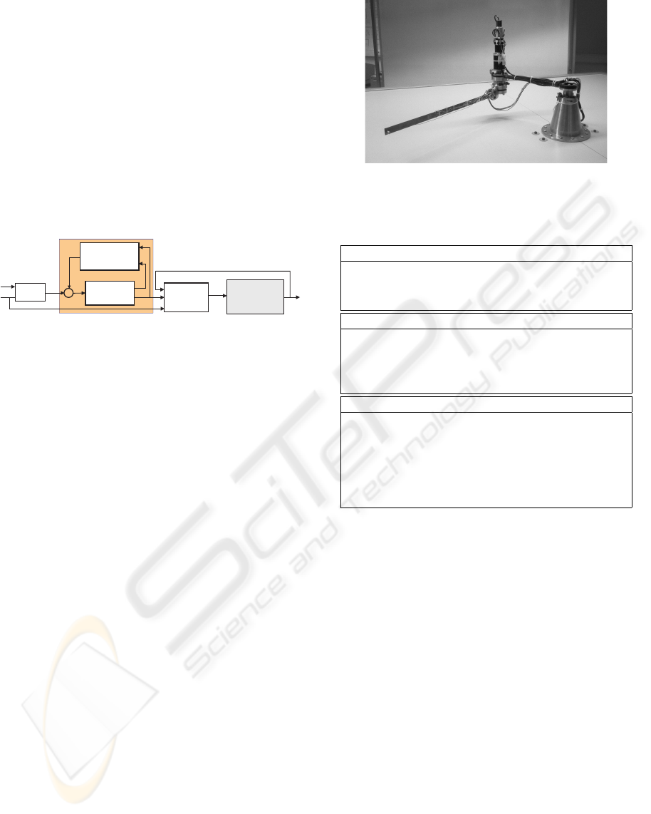
4 ROBOT EXPERIMENTAL
SETUP
For the purpose of analyze the interaction control al-
gorithm performance, an experimental setup was built
at the Robotics Laboratory. In fig. 7, a picture of the
planar flexible-link robot used for the experiments, is
presented.
Table 1 exhibits the most important physical para-
meters of the joints and links of this robot.
The control hardware used to drive the flexible ro-
bot consists of a host PC Pentium IV 3 GHz computer
that runs the Matlab/Simulink software and a target
PC Pentium 200 MHz computer, where the real-time
target software runs under the Matlab/xPC environ-
ment. The signals are processed through a low cost
ISA-bus servo I/O board from SERVO TO GO, INC.,
and the electric d.c. joint motors are driven by lin-
ear power amplifiers configured to operate as current
Figure 7: Picture of the experimental robotic setup.
Table 1: Physical parameters of the robot.
Joint 1 and rigid link 1
L
R
- link length 0.32 m
I
R
0
- Inertia of the link 0.25 kgm
2
I
m1
- Inertia of the actuator 0.093 kgm
2
Joint 2
r - Radius of the joint 0.075 m
I
H
- Rotating inertia 13.22 × 10
−4
m
4
M
H
- Mass of the joint 0.47 kg
I
m2
- Inertia of the actuator 0.024 kgm
2
Flexible link 2
L - Link length 0.5 m
e - Link thickness 0.001 m
h - Link width 0.02 m
I - Cross section inertia 1.67×10
−12
m
4
I
b
- Link inertia 99×10
−4
kgm
2
m
b
- Link mass 0.0785 kg
amplifiers. In this functioning mode, the input con-
trol signal is a voltage in the range of ±10 V with
current ratings in the interval [−3 , 3] A. The de-
flection of the elastic link is measured by three full
bridge strain gage sensors located along the link and
processed by HOTTINGER BM instrumentation am-
plifiers. The contact forces are measured by a JR
3
6-
axis force/torque sensor mounted on the contact sur-
face (see Fig. 10 for details). The force sensor hard-
ware provide decoupled and digitally filtered data at
a frequency rate of 8 KHz for each channel. Figure 8
represent the overall hardware and software control
architecture for the flexible-link robot.
5 EXPERIMENTAL RESULTS
For the purpose of analyzing the interaction control
performance, the control methodologies presented in
sections 3.1 and 3.2 are applied through experimen-
tation to the planar robot represented in fig. 7. No-
tice that all the interaction tasks described on this
ICINCO 2006 - ROBOTICS AND AUTOMATION
70

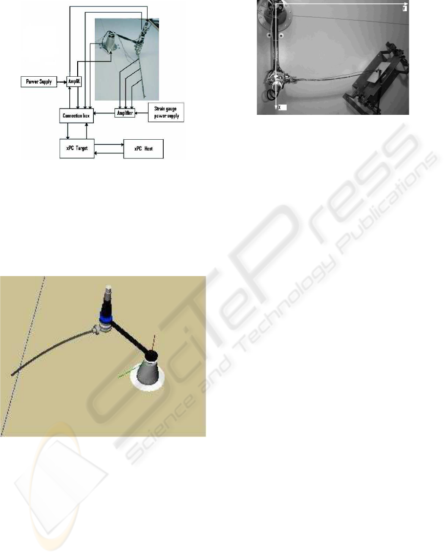
Figure 8: Hardware and software control architecture for
the flexible-link robot.
section were previously tested by simulation in Mat-
lab/Simulink in order to obtain the best performance.
For this purpose, Virtual Reality Toolbox from Mat-
lab was used to build the tridimensional (3D) robot
model, as depicted in fig. 9.
Figure 9: Picture of the 3D planar robot model built in Mat-
lab/Virtual Reality Toolbox. Notice that the dot line repre-
sents the undeformed flexible contact surface.
5.1 Rigid Surface
The first task consists of applying a force profile on
the rigid surface while maintaining the robot’s posi-
tion. In the second task, the robot should move along
the rigid surface with simultaneously application of
the desired force profile on the surface, as represented
in Fig. 10.
The sampling frequency is 1 kHz and the follow-
ing controller gains were used in all the experimental
Figure 10: Top view of the flexible robot executing an in-
teraction task.
tasks: K
P
= [2000 ; 2000] for the CLIK algorithm
and K
p
= [3000 ; 600], K
d
= [20 ; 10] for the PD
controller. Notice that all the experiments were ex-
ecuted considering that tip is already in contact with
the surface before the execution of the task.
Due to the maximum allowed values for the deflec-
tions adjusted in the robot’s supervision and control
software and the high degree of flexibility of the link,
the maximum force that is possible to apply by the
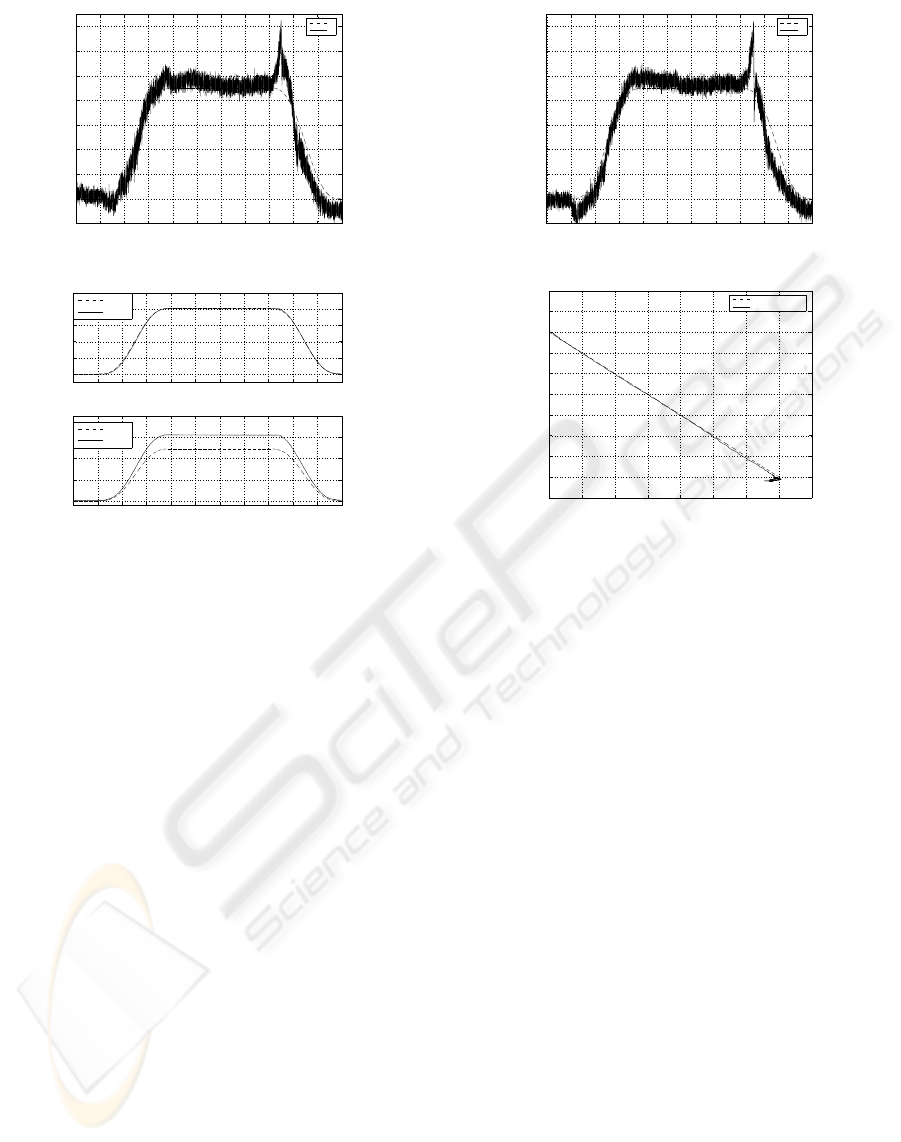
flexible link on the surface, is 1 N. In fig. 11 the re-
sults for a task where only a desired force trajectory
is applied on the surface are presented. The force is
applied at the initial contact point, P=[0.32 ; 0.575]
m. The contact surface has 45
o
of inclination with the
reference base frame x-axis. The reference force pro-
file has a maximum value of 0.9 N, a growing time of
15 seconds and a full evolution time of 50 seconds.
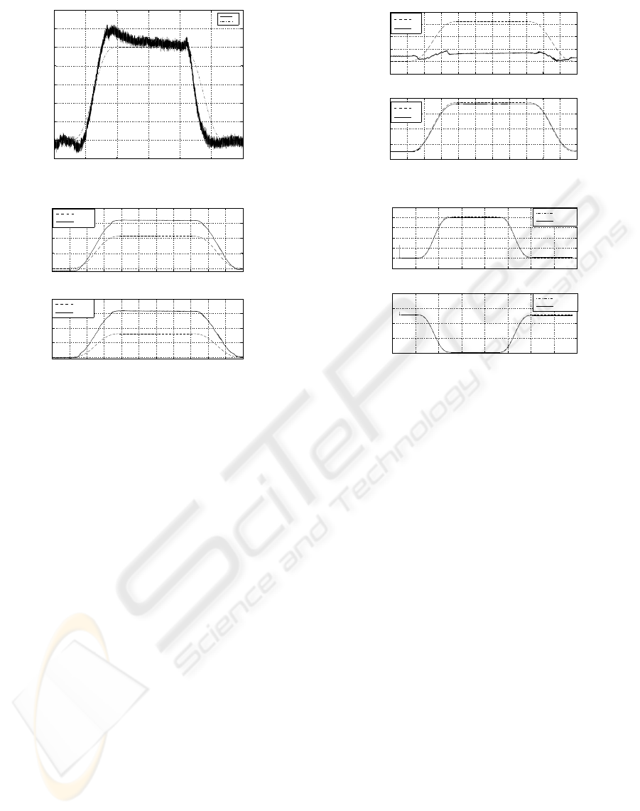
In fig. 12 the results for a task with force and posi-
tion reference trajectories are presented. The refer-
ence force has the same profile of the first task and
the position reference trajectory executes a straight
line movement with a cycloidal profile of 5 cm in 5
seconds along the rigid surface.
From the analysis of the plots, is possible to observe
a good force tracking performance in static condi-
tions (fig. 11). Also, when the robot executes a move-
ment along the rigid surface, while executing the de-
sired force profile, an acceptable force tracking per-
formance with low force errors is observed along the
trajectory (fig. 12). In all these experiments an over-
shoot is observed when the applied force begins to de-
crease, due to tip/surface contact friction effects. No-
tice that the desired force is applied on the surface
without force feedback, but the force errors are kept
small. These results validate the interaction control
strategy described in section 3.1.
5.2 Flexible Surface
In order to obtain preliminary experimental results for
a flexible environment, a soft foam was fixed on the
INTERACTION CONTROL EXPERIMENTS FOR A ROBOT WITH ONE FLEXIBLE LINK
71

80 85 90 95 100 105 110 115 120 125 130 135
−0.2
0
0.2
0.4
0.6
0.8
1
1.2
1.4
time [s]
f
d
; f [N]
Desired force vs. Actual force
fd
f
(a) Desired force vs. actual force
80 85 90 95 100 105 110 115 120 125 130 135
0
0.02
0.04
0.06
0.08
0.1
Modal amplitude
1
st
vibration mode
CLIK
Actual
80 85 90 95 100 105 110 115 120 125 130 135
0
0.05
0.1
0.15
0.2
time [s]
Modal amplitude
2
nd
vibration mode
CLIK
Actual
(b) Modal link amplitude
Figure 11: Rigid surface: contact force and modal ampli-
tudes of the flexible link.
plate attached to the force sensor. The overall esti-
mated stiffness coefficient of the device is k
e
≈110
N/m. Since the interaction controller for the flexible
surface revealed to be extremely sensitive for k
e
val-
ues larger than 15 N/m, a desired path profile f
d
with
a maximum value of 1 N was planned considering
the estimated stiffness environment but setting k
e
=15
N/m in eq. (29) in order to observe the correspondent
applied force and deformation of the environment.
From fig. 13 it is possible to observe an acceptable
force tracking behavior in static conditions. In this
case, a force overshoot is observed at the end of the
growing path due to the flexible environment charac-
teristics. From the force trajectory plot, is possible
to observe that applied force reach the desired value
of 1 N. However, since there are a significant gap be-
tween the estimated stiffness coefficient and the k
e
value used in eq. (29), the modal amplitudes of the
flexible link will not match the desired ones calcu-
lated by the CLIK algorithm (fig. 13-b). Also, due to
the k
e
mismatch described above, the cartesian trajec-
tory evolution along x−axis will exhibit a poor track-
ing performance, as depicted on fig. 14-a. Finally, is
possible to observe that joint position controller re-
veal an excellent tracking performance (see fig. 14-b
for details).
80 85 90 95 100 105 110 115 120 125 130 135
−0.2
0
0.2
0.4
0.6
0.8
1
1.2
1.4
time [s]
f
d
; f [N]
Desired force vs. Actual force
fd
f
(a) Desired force vs. actual force
0.32 0.325 0.33 0.335 0.34 0.345 0.35 0.355 0.36
0.535
0.54
0.545
0.55
0.555
0.56
0.565
0.57
0.575
0.58
0.585
x
d
; x [m]
y
d
; y [m]
Reference trajectory vs. Tip trajectory
Reference trajectory
Tip trajectory
(b) x − y trajectory evolution
Figure 12: Rigid surface: contact force and cartesian trajec-
tory along the surface.
6 CONCLUSIONS
In this article interaction control strategies for a ma-
nipulator robot with a two degrees of mobility and a
flexible link were analyzed by simulation and exper-
imentation. The interaction control results reveal the
successful implementation of the control algorithms
in real-time for a robot with one flexible link. The
interaction control results were obtained considering
rigid and flexible contact surfaces.
Future research will concentrate on the improvement
of the real-time software functionality, the study of
more complex inverse kinematic algorithms for flexi-
ble arms and the improvement of the interaction con-
troller robustness for the flexible contact surface.
ACKNOWLEDGEMENTS
The authors would like to thank to Professors Bruno
Siciliano and Luigi Villani for their support during the
CLIK algorithm implementation in Matlab/Simulink.
ICINCO 2006 - ROBOTICS AND AUTOMATION
72

80 90 100 110 120 130 140
−0.2
0
0.2
0.4
0.6
0.8
1
1.2
1.4
time [s]
f
d
; f [N]
Desired force vs. actual force
f
fd
(a) Desired force vs. actual force
80 85 90 95 100 105 110 115 120 125 130 135
0
5
10
15
20
x 10
−3
Modal amplitude
1
st
vibration mode
CLIK
Actual
80 85 90 95 100 105 110 115 120 125 130 135
0
0.01
0.02
0.03
0.04
2
nd
vibration mode
time [s]
Modal amplitude
CLIK
Actual
(b) Modal link amplitude
Figure 13: Flexible surface: contact force and modal ampli-
tudes of the flexible link.
REFERENCES
Canudas de Wit, C., Siciliano, B., and Bastin, G. (1998).
Theory of Robot Control. Springer Verlag.
Cheong, J., Chung, W. K., and Youm, Y. (2004). Inverse
kinematics of multilink flexible robots for high-speed
applications. IEEE Transactions on Robotics and Au-
tomation, 20(2):269–282.
Khorrami, F. and Jain, S. (1994). Nonlinear control with
end-point acceleration feedback for a two-link flexible
manipulator: experimental results. Journal of Robotic
Systems, 11:591–603.
Martins, J. (2000). Modeling and identification of flexible
manipulators towards robust control. Master’s the-
sis, Universidade T
´
ecnica de Lisboa, Instituto Supe-
rior T
´
ecnico, Lisbon.
Nabais, J. (2002). Sliding model control of a flexible link
robot (in portuguese). Master’s thesis, Universidade
T
´
ecnica de Lisboa, Instituto Superior T
´
ecnico, Lis-
bon.
Siciliano, B. (1990). A closed-loop inverse kinematic
scheme for on-line joint based robot control. Robot-
ica, 8:231–243.
Siciliano, B. (1999). Closed-loop inverse kinematics al-
gorithm for constrained flexible manipulators under
gravity. Journal of Robotics Systems, 16:353–362.
80 85 90 95 100 105 110 115 120 125 130 135
0.318
0.32
0.322
0.324
0.326
0.328
x
d
; x [m]
Desired x
d
vs. actual x
80 85 90 95 100 105 110 115 120 125 130 135
0.574
0.576
0.578
0.58
0.582
time [s]
y
d
; y [m]
Desired y
d
vs. actual y
x
d
x
y
d
y
(a) Desired trajectory vs. actual trajectory
70 80 90 100 110 120 130 140 150
−0.005
0
0.005
0.01
0.015
0.02
0.025
q
CLIK
; q [rad]
q CLIK vs. q Real J.1
q CLIK
q actual
70 80 90 100 110 120 130 140 150
1.52
1.54
1.56
1.58
1.6
q CLIK vs. q Real J.2
time [s]
q
CLIK
; q [rad]
q CLIK
q actual
(b) CLIK reference angles vs. actual an-
gles
Figure 14: Flexible surface: Cartesian and joint trajectories.
Siciliano, B. and Villani, L. (2001). An inverse kinematics
algorithm for interaction control of a flexible arm with
a compliant surface. Control Engineering Practice,
9:191–198.
Talebi, H., Khorasani, K., and Patel, R. (1998). Neural
network based control schemes for flexible-link ma-
nipulators: simulations and experiments. Neural Net-
works, 11:1357–1377.
Vandegrift, M., Lewis, F., and Zhu, S. (1994). Flexible-link
robot arm control by feedback linearization/singular
perturbation approach. Journal of Robotic Systems,
11:591–603.
Zeng, G. and Hemami, A. (1997). An overview of robot
force control. Robotica, 15:473–482.
INTERACTION CONTROL EXPERIMENTS FOR A ROBOT WITH ONE FLEXIBLE LINK
73