A MODEL PREDICTIVE CONTROLLER BASED ON SUPPORT
VECTOR REGRESSION AND GENETIC OPTIMIZATION FOR
AN SP-100 SPACE NUCLEAR REACTOR
Man Gyun Na
Nuclear Engineering Department, Chosun University, Gwangju 501-759, Republic of Korea
Belle R. Upadhyaya
Nuclear Engineering Department, The University of Tennessee, Knoxville, Tennessee 37996-2300, U.S.A.
Keywords: Genetic algorithm, Model predictive control, Reactor power control, SP-100 space reactor, and Support
vector machines.
Abstract: In this work, a model predictive control (MPC) method combined with support vector regression (SVR), is
applied to the design of the thermoelectric (TE) power control in the SP-100 space reactor. The future TE
power is predicted by using SVR. The objectives of the proposed model predictive controller are to
minimize both the difference between the predicted TE power and the desired power, and the variation of
control drum angle that adjusts the control reactivity. Also, the objectives are subject to maximum and
minimum control drum angle and maximum drum angle variation speed. The genetic algorithm (GA) is
used to optimize the model predictive controller. A lumped parameter simulation model of the SP-100
nuclear space reactor is used to verify the proposed controller. The results of numerical simulations to check
the performance of the proposed controller show that the TE generator power level controlled by the
proposed controller could track the target power level effectively, satisfying all control constraints.
1 INTRODUCTION
The SP-100 was designed to provide a realistic and
reliable source of long-term power for space
exploration and exploitation activities. The SP-100
system is a fast spectrum lithium-cooled reactor
system with an electric power rating of 100 kW
(Demuth, 2003) and its energy conversion system is
based on a direct TE conversion mechanism. The
control system is a key element of space reactor
design to meet the mission requirements of
economics, reliability, safety, survivability, and life
expectancy. For a space mission with uncertain
environment, rare events, and communication
delays, all the control functions must be achieved
through a sophisticated control system with a limited
degree of human intervention from the earth.
In order to optimize the reactor power control
performance, techniques for the optimal power
control of nuclear reactors have been studied
extensively in the past two decades (Cho and
Grossman, 1983; Shtessel, 1998). But it is very
difficult to design optimized controllers for nuclear
systems because of variations in nuclear system
parameters and modeling uncertainties, and in
particular, for the long-term operation of the SP-100
reactor.
This work employs the MPC method, which has
received much attention as a powerful tool for the
control of industrial process systems (Kwon and
Pearson, 1977; Garcia et al., 1989). The basic
concept of the model predictive control is to solve an
optimization problem for a finite future at the
current time. Once a future input trajectory is
chosen, only the first element of that trajectory is
applied as the input to the plant, and the calculation
is repeated at each subsequent instant. This method
has many advantages over the conventional infinite
horizon control because it is possible to handle input
and output constraints in a systematic manner during
the design and implementation of the control. In
particular, it is a suitable control strategy for
nonlinear time varying systems. The MPC method
136
Gyun Na M. and R. Upadhyaya B. (2006).
A MODEL PREDICTIVE CONTROLLER BASED ON SUPPORT VECTOR REGRESSION AND GENETIC OPTIMIZATION FOR AN SP-100 SPACE
NUCLEAR REACTOR.
In Proceedings of the Third International Conference on Informatics in Control, Automation and Robotics, pages 136-141
DOI: 10.5220/0001205301360141
Copyright
c
 SciTePress

has been applied to a nuclear engineering problem
(Na et al., 2003).
Also, this work incorporates the support vector
machines (SVMs) that have been successfully
employed to solve nonlinear regression problems
(Pai and Hong, 2005; Yan et al., 2004). The SVR is
used to predict the future output that is required in
the optimization objective of the model predictive
control. That is, at the present time the behavior of
the process over a prediction horizon is considered
and the process output to changes in the manipulated
variable is predicted by SVMs. In this application,
based on this identified reactor model that consists
of the control drum angle and the TE generator
power, the future TE generator power is predicted.
The objective function for MPC is minimized by a
GA that is widely used for optimization problems. A
lumped parameter simulation model of the SP-100
space reactor is used to verify the proposed
controller for a space nuclear reactor.
2 MPC CONTROLLER USING
SVR
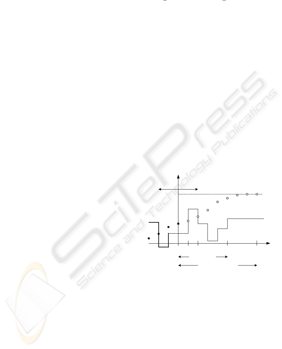
Figure 1 shows the basic concept of the model
predictive control (Garcia, 1989). At first a set of
present and future control moves are assumed, and
the future behavior of the process outputs can be
predicted over a prediction horizon
L with the
assumed present and future control moves. Then the
optimized
M
present and future control moves
(
M
L≤ ) are optimized to minimize a quadratic
objective function. Although
M
optimized control
moves are calculated, only the first control move is
implemented. At the next time step, new values of
the measured output are obtained, the control
horizon is shifted forward by one step, and the same
calculations are repeated by using updated
measurements.
The purpose of taking new measurements at each
time step is to compensate for unmeasured
disturbances and model inaccuracies, both of which
cause the measured system output to be different
from the predicted one. At every time instant, model
predictive control requires the on-line solution of an
optimization problem to compute optimal control
inputs over a fixed number of future time instants,
known as the time horizon.
Also, in order to achieve fast responses and
prevent excessive control effort, the associated
performance index for deriving an optimal control
input is represented by the following quadratic
function:
[]
22
11
11
ˆ
(|)() ( 1)
22
LM
kk
Jytktztk utk ρ
==
=+−++Δ+−
⎡⎤
⎣⎦
∑∑
(1)
min max
max max
(1)0 for
subject to constraints ( )
()
ut k k M
uutu
du u t du
Δ
+− = >
⎧
⎪
≤≤
⎨
⎪
−≤Δ≤
⎩
where the parameter
ρ
determines trade-off
between the TE power (system output) error and
control drum angle (control input) move between
neighbouring time steps, and
z
is a setpoint (desired
TE power). The estimate
ˆ
(|)yt k t+
is an optimum
k -step-ahead prediction of the system output based
on data up to time
t
. u
Δ
, )1()()(
−
−=Δ tututu , is
an input move between neighbouring time steps. The
parameters
L
and
M
are called the prediction
horizon and the control horizon, respectively. The
prediction horizon represents the limit of the instant
in which it is desired for the output to follow the
reference sequence. The constraint,
(1)0ut kΔ+−=
for
kM> , means that there is no variation in the
control signals after a certain interval
M
.
t
1t
+
1tM+−
tL+
Control Horizon
Prediction Horizon
FuturePast
""
Predicted Outputs
ˆ
(|)yt k t+
Control Inputs
(|)ut k t
+
Reference Trajectory
z
Figure 1: Basic concept of a MPC method.
In order to obtain control inputs, the predicted
outputs are first calculated by function
approximation using SVMs, in which inputs consist
of past values of control system inputs and outputs
and of future control system input signals. Along
with the introduction of Vapnik’s
ε
-insensitive loss
function (Vapnik, 1995), SVMs also have been
extended and widely used to solve nonlinear
regression estimation problems. In SVM regression
the concept is to map the input data into a high
dimensional feature space and subsequently carry
out the linear regression in the feature space.
A MODEL PREDICTIVE CONTROLLER BASED ON SUPPORT VECTOR REGRESSION AND GENETIC
OPTIMIZATION FOR AN SP-100 SPACE NUCLEAR REACTOR
137

Therefore, the SVM regression is used to predict the
future output based on past inputs and outputs.
2.1 Output Prediction
The basic concept of the SVM regression is to map
nonlinearly the original data
x into a higher
dimensional feature space. Hence, given a set of data
{}
N
i
ii
y
1
),(
=
x where
i
x is the input vector,
i
y is the
actual output value and
N is the total number of
data patterns, the SVM regression function is
bwfy
T
N
i
ii
+===
∑
=
)()()(
1
xφwxx φ
, (2)
where
)(x
i
φ
is called the feature that is nonlinearly
mapped from the input space
x ,
[]
T
N
www "
21
=w
, and
[]
T
N
φφφ "
21
=φ
.
The parameters
w and b are a support vector
weight and a bias that are calculated by minimizing
the following regularized risk function:
∑
=
−+=
N
i
i
T
fyR
1
)(
2
1
)(
ε
λ xwww , (3)
where
⎪
⎩
⎪
⎨
⎧
−−
<−
=−
otherwise)(
)(0
)(
ε
ε
ε
x
x
x
fy
fy
fy
i
i
i
(4)
Here,
λ
and
ε
are user-specified parameters and
ε
)(xfy
i
− is called the
ε
-insensitive loss function
(Vapnik, 1995). The loss equals zero if the estimated
value is within an error level
ε
. The regularized risk
function can be rewritten by the following
constrained form:
()
∑
=
++=
N
i
ii
T
R
1
*
2
1
*),,(
ξξλ wwξξw , (5)
subject to the constraints
⎪
⎩
⎪
⎨
⎧
=≥
=+≤−+
=+≤−−
Ni
Niyb
Niby
ii
ii
T
i
T
i
,,2,1,0,
,,2,1,)(
,,2,1,)(
*
*
"
"
"
ξξ
ξε
ξε
xφw
xφw
where the constant
λ
determines the trade-off
between the flatness of
)(xf and the amount up to
which deviations larger than
ε
are tolerated and
[]
T
N
ξξξ "
21
=ξ ,
[]
T
N
ξξξ "
21
*
=ξ are
slack variables representing upper and lower
constraints on the outputs of the system.
The solution to the constrained optimization
problem is given by the saddle point of the Lagrange
functional:
(
)
() []
[]
()
∑∑
∑∑
==
==
+−++−−−
++−+−++
=Φ
N
i
iiii
N
i
ii
T
ii
N
i
iii
T
i
N
i
ii
T
iiiiii
by
yb
b
1
**
1
**
11
*
***
)(
)(
2
1
,,,,,,,
ξβξβξεα
ξεαξξλ
ξξααξξ
xφw
xφwww
w
(6)
The above equation is minimized with respect to
the primal variables
*
,,,
ii
b ξξ w , and then
maximized with respect to the nonnegative
Lagrangian multipliers
**
,,,
iiii
ββαα . The
minimum with respect to
*
,,,
ii
b ξξ w provides the
following conditions:
()
)(
1
*
i
N
i
ii
xφw
∑
=
−= αα
, (7)
()
0
1
*
=−
∑
=
N
i
ii
αα ,
Ni
ii
,,2,1,0 "
=
=
−
−
β
α
λ
,
Ni
ii
,,2,1,0
**
"==−− βαλ .
The Lagrange functional can be rewritten by
using the above minimum conditions as follows:
() ( ) ( )
()( ) ()
)(
2
1
,
11
**
1
*
1
**
ji
T
N
i
N
j
jjii
N
i
ii
N
i
iiiii
y
xφxφ
∑∑
∑∑
==
==
−−−
+−−=Ψ
αααα
ααεαααα
(8)
subject to the constraints
()
Ni
ii
N
i
ii
,,1,0,0,0
*
1
*
"=≤≤≤≤=−
∑
=
λαλααα
(9)
By solving the above equation with standard
quadratic programming technique, the values of
*
,
ii
αα are found out. By substituting Eq. (7) into
Eq. (2), the regression function becomes
()
()
bK
bfy
N
i
iii
i
T
N
i
ii
+−=
+−==
∑
∑
=
=
1
*
1
*
),(
)()()(
xx
xφxφx
αα
αα
(10)
ICINCO 2006 - INTELLIGENT CONTROL SYSTEMS AND OPTIMIZATION
138

where
)()(),( xφxφxx
i
T
i
K =
is called the kernel
function. A number of coefficients
*
ii
αα − are
nonzero values and the corresponding training data
points have approximation error equal to or larger
than
ε
. They are called support vectors.
2.2 Objective Function Optimization
by a GA
The objective function of Eq. (1) can be solved by
linear matrix inequality (LMI) techniques. In this
work, a GA is used to minimize the objective
function with multiple objectives. The GA has been
known to be effective in solving multiple objective
functions and is less susceptible to getting stuck at
local minima compared to conventional search
methods (Goldberg, 1989).
We propose an SVM-based MPC methodology
which is based on a dynamic nonlinear SVM model
of the SP-100 space reactor. The optimization
problem which needs to be solved online is no
longer a linear problem but a complicated nonlinear
problem which requires a tremendous computational
effort. This calculation cannot be completed on time
even by the fast computing systems [22]. Due to the
peculiarity of the SVM model, conventional
optimization techniques cannot be easily applied.
Therefore, in this work, the online optimization
problem is solved using a GA.
In the GA, the term
chromosome is referred to as
a candidate solution that minimizes a cost function.
The GAs require a fitness function and the fitness
function evaluates the extent to which each
candidate solution is suitable for specified
objectives. The GA starts with an initial population
of chromosomes, which represent possible solutions
of the optimization problem. The fitness function is
computed for each chromosome. New generations
are produced by the genetic operators, such as
selection, crossover, and mutation. The algorithm
stops after the maximum allowed time has elapsed.
A chromosome which is a candidate solution of
the optimization problem is represented by
g
s
,
whose elements consist of present and future control
inputs and has the following structure (Sarimveis
and Bafas, 2003):
() ( 1) ( 1)
gg g g
sutut utM
⎡⎤
=++−
⎣⎦
"
, (11)
where
t indicates the current time. Assuming we
have chosen the number of chromosomes
G , which
will constitute the initial population, the crossover
probability
c
p and the mutation probability
m
p , the
algorithm proceeds according to the following steps:
Step 1 (initial population generation): Set the
number of iterations
1iter
=
. Generate an initial
population consisting of a total of
G chromosomes.
The values are allocated randomly, but they should
satisfy both input and input move constraints of Eq.
(1).
Step 2 (fitness function evaluation): Evaluate the
objective function of Eq. (1) for all the chosen
chromosomes. Then invert the objective function
values and find the total fitness of the population as
follows:
1
1
()
G
g
g
F
J
t
=
=
∑
, (12)
where
()
g
J
t
is the objective function value for the
g
-th chromosome and the inversion of ()
g
J
t is a
fitness value of the
g
-th chromosome. Then,
calculate the normalized fitness value of each
chromosome, meaning that the selection of
probability
g
p calculated by
(
)
1/ ( )
,1,,
g
g
Jt
pgG
F
==" . (13)
Step 3 (selection operation): Calculate the
cumulative probability
g
q
for each chromosome
using the following equation:
1
,1,,
g
gj
j
qpg G
=
==
∑
" . (14)
For
1, ,
g
G
=
" , generate a random number
r
between 0 and 1. Select the chromosome for which
1
g
g
qrq
−
≤
≤
. At this point of the algorithm a new
population of chromosomes has been generated. The
chromosomes with high fitness value have more
chance to be selected.
Step 4 (crossover operation): For each
chromosome
g
s
, generate a random number
r
between 0 and 1. If
r
is lower than
c
p , this
particular chromosome will undergo the process of
crossover, otherwise it will remain unchanged. Mate
the selected chromosomes. The crossing point is the
position indicated by a random integer number
z
generated between 0 and
1
M
−
. Two new
chromosomes are produced by interchanging all the
members of the parents following the crossing point.
The crossover operation might produce infeasible
offsprings and this situation is avoided by a simple
correction mechanism for an input variable, which
modifies the values of the input parameters after the
A MODEL PREDICTIVE CONTROLLER BASED ON SUPPORT VECTOR REGRESSION AND GENETIC
OPTIMIZATION FOR AN SP-100 SPACE NUCLEAR REACTOR
139

cross position so that the input move constraints are
satisfied.
Step 5 (mutation operation): For every member
of each chromosome
g
s
, generate a random number
r
between 0 and 1. If
r
is lower than
m
p , this
particular member of the chromosome will undergo
the process of mutation, otherwise it will remain
unchanged. Each chromosome should satisfy both
input and input move constraints of Eq. (1) after
mutation.
Step 6 (repeat or stop): If the maximum allowed
time has not expired, set
1 iter iter=+ and return
the algorithm to Step 2. Otherwise, stop the
algorithm and select the chromosome that produced
the lowest value of the objective function throughout
the entire procedure.
3 APPLICATION TO THE SP-100
SPACE NUCLEAR REACTOR
The SP-100 system is a fast spectrum lithium-cooled
reactor system that can generate electric power of
100 kW for space exploration and exploitation
activities. The reactor system is made up of a reactor
core, a primary heat transport loop, a thermoelectric
generator, and a secondary heat transport loop to
reject waste heat into space through radiators. The
reactor core is composed of small disks of highly
enriched (93%) uranium nitride fuel contained in
sealed tubes. The heat generated in the reactor core
is transported by liquid lithium and is circulated by
electromagnetic (EM) pumps. The interface between
the primary heat transport system and the energy
conversion system is a set of primary heat
exchangers. The energy conversion system uses the
direct TE conversion mechanism. A temperature
drop of about 500 K is maintained across the TE
elements by the cooling effect of a second liquid
lithium loop that transfers the waste heat from the
converter to a heat-pipe radiator.
The model predictive controller for the power
level control is subject to constraints as follows:
(1)0forut j j MΔ+−= >, 0()180
oo
ut≤≤ ,
() 1.4
o
utΔ≤.
The sampling interval
T
is 1 second. The external
reactivity control uses the mechanism of the stepper
motor control drum system (Shtessel, 1998).
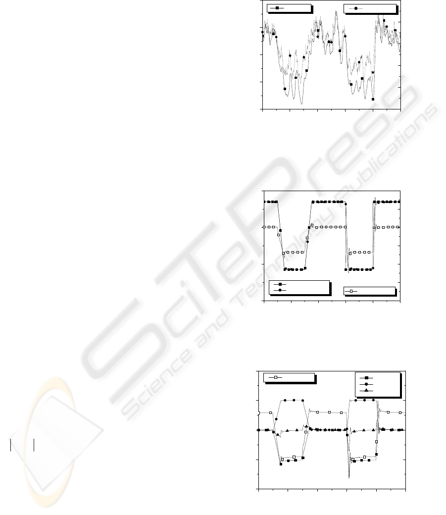
The regression function by SVMs is solved by
using one fifth of a data set shown in Fig. 2. 77
support vectors are collected at every interval (one
per five data points) from the data of 1000 sampling
points.
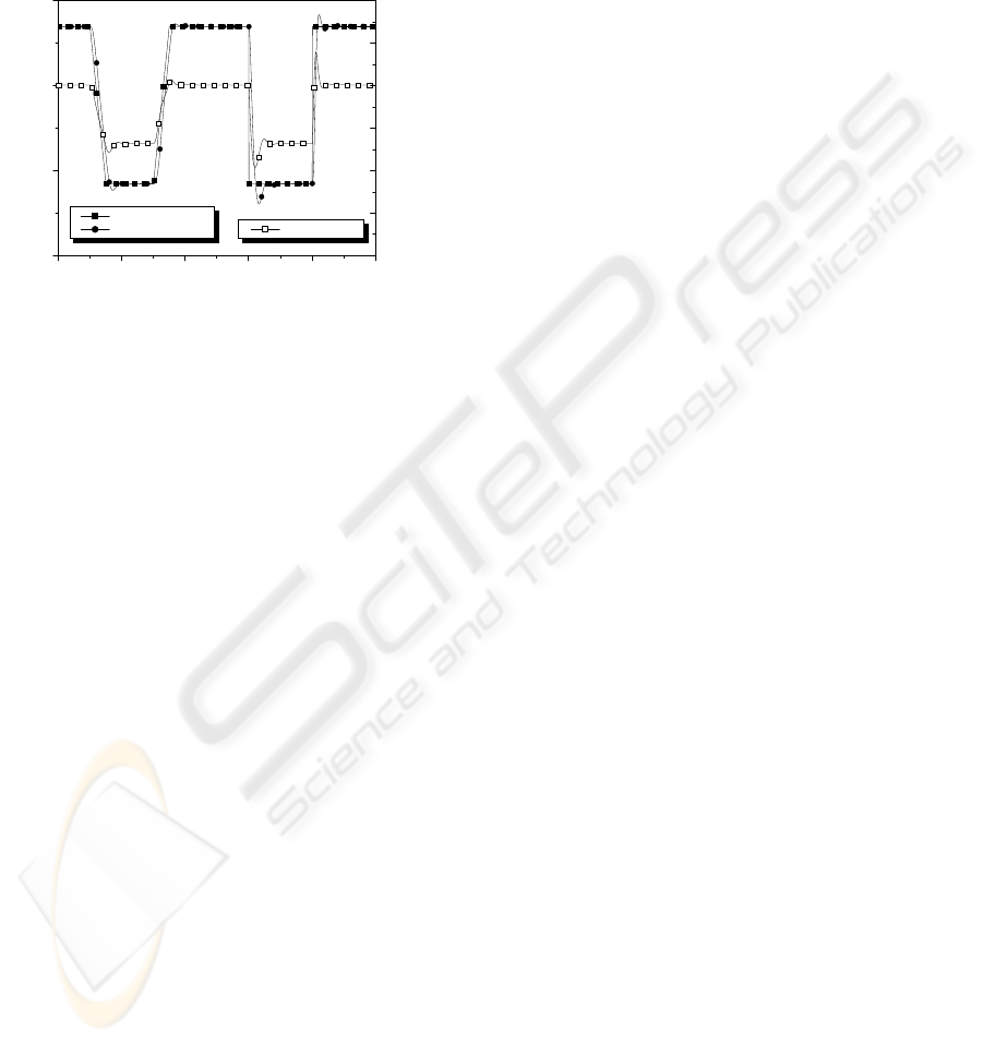
Figure 3 shows the detailed performance of the
proposed model predictive controller. It is shown
that the TE generator power follows its desired value
very well. It was known that the proposed controller
meets several constraints very well and
accomplishes the fast and stable responses.
0 200 400 600 800 1000
30
60
90
120
150
Drum angle (deg)
TE electric power (KW)
time (sec)
TE power
90
100
110
120
130
140
drum angle
Figure 2: Training data plot.
0 200 400 600 800 1000
30
60
90
120
TE power (KW)
time (sec)
TE demand power
TE power
0.0
0.5
1.0
1.5
2.0
2.5
3.0
thermal reactor power (MW)
thermal power
(a) TE power and thermal reactor power
0 200 400 600 800 1000
100
110
120
130
140
drum angle
control drum angle (deg)
time (sec)
-1.0
-0.5
0.0
0.5
1.0
reactivity (dollars)
control
feedback
total
(b) control drum angle and reactivity
Figure 3: Performance of the proposed MPC controller.
ICINCO 2006 - INTELLIGENT CONTROL SYSTEMS AND OPTIMIZATION
140

In addition, a conventional proportional-integral
(PI) controller was designed to compare the
performance of the power level response with the
proposed model predictive controller optimized by
the GA (refer to Fig. 4). The PI controller has a little
slower response and bigger overshoot and
undershoot than the proposed MPC.
0 200 400 600 800 1000
30
60
90
120
thermal reactor power (MW)
TE power (KW)
time(sec)
TE demand power
TE power
0.0
0.5
1.0
1.5
2.0
2.5
3.0
reactor power
Figure 4: Performance of a PI controller.
4 CONCLUSIONS
In this work, the model predictive controller
optimized by the GA and combined by SVMs was
developed to control the nuclear power in the SP-
100 space reactor system. The future TE power is
predicted by using the SVMs and the GA was used
to optimize the model predictive controller. It was
determined from many numerical simulation results
that the proposed controller was able to actuate the
control drum to regulate the control reactivity so that
the TE generator electric power followed the set
point changes according to load demands. Also, the
performance of the new proposed controller was
proved to be more efficient than that of the
conventional PI controller.
ACKNOWLEDGEMENTS
The research is supported in part by Korea MOST
(Ministry of Science and Technology) BAERI grant
and in part by a U.S. Department of Energy NEER
grant (DE-FG07-04ID14589) with the University of
Tennessee.
REFERENCES
Cho, N.Z., Grossman, L.M., 1983. Optimal Control for
Xenon Spatial Oscillations in Load Follow of a
Nuclear Reactor. Nucl. Sci. Eng., Vol. 83, pp. 136-
148.
Demuth, S.F., 2003. SP-100 Space Reactor Design.
Progress in Nuclear Energy, Vol. 42, No. 3, pp. 323-
359.
Garcia, C.E., Prett, D.M., Morari, M., 1989. Model
Predictive Control: Theory and Practice – A Survey.
Automatica, Vol. 25, No. 3, pp. 335-348.
Goldberg, D.E., 1989. Genetic Algorithms in Search,
Optimization, and Machine Learning, Addison
Wesley, Reading, Massachusetts.
Kwon, W.H., Pearson, A.E., 1977. A Modified Quadratic
Cost Problem and Feedback Stabilization of a Linear
System. IEEE Trans. Automatic Control, Vol.22, No.
5, pp. 838-842.
Na, M.G., Shin, S.H., Kim, W.C., 2003. A Model
Predictive Controller for Nuclear Reactor Power. J.
Korean Nucl. Soc., Vol. 35, No. 5, pp. 399-411.
Pai, P.-F., Hong, W.-C., 2005. Support Vector Machines
with Simulated Annealing Algorithms in Electricity
Load Forecasting. Energy Conversion and
Management, Vol. 46, pp. 2669-2688.
Sarimveis, H., Bafas, G., 2003. Fuzzy Model Predictive
Control of Non-linear Processes Using Genetic
Algorithms. Fuzzy Sets Systems, Vol. 139, pp. 59-80.
Shtessel, Y.B., 1998. Sliding Mode Control of the Space
Nuclear Reactor System. IEEE Trans. Aerospace and
Electronic Systems, Vol. 34, No. 2, pp. 579-589.
Vapnik, V., 1995. The Nature of Statistical Learning
Theory, Springer, New York.
Yan, W., Shao, H., Wang, X., 2004. Soft Sensing
Modeling Based on Support Vector Machine and
Bayesian Model Selection. Computers and Chemical
Engineering, Vol. 28, pp. 1489-1498.
A MODEL PREDICTIVE CONTROLLER BASED ON SUPPORT VECTOR REGRESSION AND GENETIC
OPTIMIZATION FOR AN SP-100 SPACE NUCLEAR REACTOR
141