DESIGN OF AN ITERATIVE LEARNING CONTROL FOR A SERVO

SYTEM USING MULTI-DICTIONARY MATCHING PURSUIT

Iuliana Rotariu

ARC Centre of Excellence for Autonomous Systems, University of Sydney

NSW2006, Sydney, Australia

Erik Vullings

MELCOE, Macquarie University

NSW2109, Sydney, Australia

Keywords:

Iterative Learning Control, System Dynamics, Mechatronics, Time-frequency analysis, Wigner distribution,

Atomic decomposition, Matching Pursuit.

Abstract:

Many motion systems repeatedly follow the same trajectory. However, in many cases, the motion system does

not learn from tracking errors obtained in a previous cycle. Iterative Learning Control (ILC) resolves this

issue by compensating for previous tracking errors, but it suffers from not being able to distinguish between

tracking errors caused by machine dynamics versus errors caused by noise, and by trying to ’learn’ the noise,

additional errors are introduced.

In this paper we address this issue by using the servo error signal by identifying the time-varying nonlinear

effects, which can be learned and therefore improve the position accuracy, versus the stochastic effects, which

cannot be learned. The identiﬁcation of these effects is performed by means of time-frequency analysis of

the servo error and therefore our goal is to obtain a high-resolution time-frequency energy distribution of the

analyzed signal. Here we compare the servo error energy distribution by three means: (1) Wigner distribution;

(2) adaptive signal decomposition over one dictionary of modulated versions of wavelets (simple atomic dic-

tionary); (3) and by means of combining several simple atomic dictionaries into a complex atomic dictionary.

We show that the latter approach leads to the highest-resolution energy distribution and tracking performance.

1 INTRODUCTION

The wafer scanner mechatronic motion system is an

opto-mechanical machine for producing Integrated

Circuits (ICs) on a silicon wafer using a photolitho-

graphic process. One of the main components of a

wafer scanner is the six degrees of freedom (DOF’s)

wafer stage (Rotariu et al., 2003a). This is an electro-

mechanical servo system that positions the wafer

(200-300mm diameter) with respect to the imag-

ing optics. The wafer stage largely determines the

throughput (80-100 wafers/h, 80-200 ICs/wafer) and

the accuracy of the products, and they are both sub-

ject to severe performance requirements. Normal scan

speeds and accelerations are 0.5 m/s and 10 m/s

, re-

spectively. In order to maximize the throughput and

minimize the servo error of such a complex dynamical

system, advanced intelligent identiﬁcation and con-

trol schemes are preferred to standard linear or robust

non-linear techniques (Casalino and Bartolini, 1984).

One of such advanced intelligent control schemes,

Iterative Learning Control (ILC), is an effective tech-

nique to reduce systematic control errors that occur in

systems that repetitively perform the same motion or

operation (Moore, 1993).

Although the time-domain ILC results can be ex-

tended to time-varying and nonlinear systems (Goh,

1994), the time-domain analysis does not give use-

ful frequency domain insights for the learning design.

In addition, the time-domain analysis results do not

address the issue of good transients and long-term

stability, and while different schemes for tuning of

the learning gain (Chang et al., 1992) have been pro-

posed, in (Wirkander and Longman, 1999) it has been

pointed out that the learning gain is not a critical fac-

tor to bandwidth. On the other hand, many frequency

domain analysis ILC algorithms have been proposed

based on frequency response methods and iteration

varying ﬁlter schemes (Tang et al., 2000), (Norrl

of,

2002), but these do not give insightful time-domain

information for the learning design or they depend

heavily on the system model.

A logical advance of the above-mentioned time-

based and frequency-based ILC methods is to use

an ILC based on time-frequency analysis of control

signals. This has been ﬁrst proposed in (Chen and

Rotariu I. and Vullings E. (2006).

DESIGN OF AN ITERATIVE LEARNING CONTROL FOR A SERVO SYTEM USING MULTI-DICTIONARY MATCHING PURSUIT.

In Proceedings of the Third International Conference on Informatics in Control, Automation and Robotics, pages 24-31

DOI: 10.5220/0001206400240031

 SciTePress

Moore, 2001), where an adaptive scheme of learning

feedforward control based on a B-spline network is

presented. In (Zhang et al., 2005) the use of wavelet

packet transform for time-frequency analysis and de-

sign of a cutoff frequency tuning for the ILC scheme

is proposed. In (Zheng and Alleyne, 2001), (Ro-

tariu et al., 2003a) continuous Wigner transform is

used to analyze the signals and in (Tharayil and Al-

leyne, 2004) and (Rotariu et al., 2006) an adaptive

robustness ﬁlter based on quadratic time-frequency

analysis (Wigner distribution) of the control signals

is proposed. In case of the Wigner distribution, exten-

sive studies have been made and methods (Cappellini

and Constantinides, 1984), (Rotariu et al., 2006) de-

vised to remove the cross-terms in some way, but

these methods do not improve the frequency resolu-

tion. Therefore, we have to focus on alternative meth-

ods that do increase the frequency resolution and re-

duce the cross-terms as well.

In this paper we propose an adaptive ILC based on

high-resolution time-frequency analysis of the con-

trol signals which is performed by means of signal

decomposition over a simple versus a complex time-

frequency atomic dictionary. We shall show that our

analysis in these two cases leads to a better under-

standing of the systems dynamics and more insightful

learning information than (piecewise) Wigner-based

adaptive ILC, while achieving a very good tracking

performance.

In Section II, the results of the signal analysis by

means of Wigner distribution will be used to ﬁnd a

suitable proﬁle for the bandwidth of the time-varying

robustness ﬁlter. In the end of this section it will be-

come clear that by increasing the resolution and accu-

racy of the time-frequency distribution, the tracking

performance of the ILC improves. In order to achieve

this, in Section 2.2 we shall introduce another two dif-

ferent time-frequency analysis methods of the servo

error signal than Wigner distribution; as consequence,

in Section 2.2 we shall show that the design of the

adaptive ILC changes and that this leads to very good

tracking performance of the proposed learning algo-

rithm.

2 TIME-FREQUENCY ADAPTIVE

ILC

This section discusses the time-frequency adaptive

ILC, i.e. time-varying adaptive ILC whose design is

based on quadratic time-frequency representation of

the control signals. Intuitively, this means that the

ILC ’gain’ is governed by the dynamics still present

in the error signal after the previous iteration: high

dynamic behavior leads to a large gain, low dynamic

behavior (noise) is ignored.

2.1 Time-varying Adaptive ILC

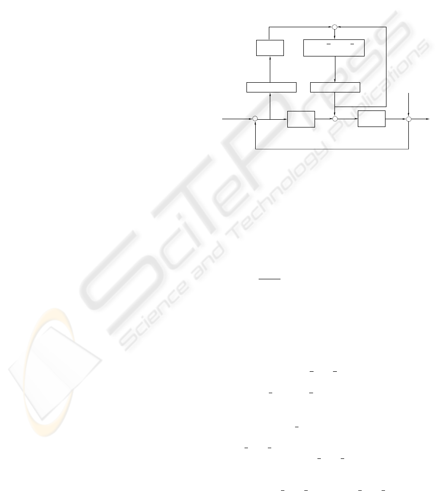
In this section the concept of time-varying adaptive

ILC is introduced (see Figure 1). We restrict the study

to the case where the plant is a causal, LTI dynamical

system P . C is a feedback controller which insures

the stability of the closed loop system.

We suppose that the desired response r is deﬁned on

the interval (t

, t

), where t

≤ ∞ and the initial

conditions are the same at the beginning of each iter-

ation.

−

k+1

Q(·,

t, Ω

(t))

error table

FF table

Figure 1: A block schematic for adaptive ILC.

The goal of the ILC design is to ﬁnd the feed-

forward signal u

∗

such that r = P u

∗

. We seek

a sequence of inputs u

with the property that

lim

k→∞

= u

∗

, where the index k is the iteration.

The adaptive ILC design consists of the design of

the L and Q ﬁlters. The learning ﬁlter L is the same

as for standard ILC, i.e. it has to approximate a sta-

ble inverse of the modeled process sensitivity function

(s) =

1+P C

(Rotariu et al., 2004).

The process sensitivity function as steady-state

transfer function is measured at the center wafer po-

sition and it does not account for system’s position

dependent dynamics within the scanning trajectory

(Rotariu et al., 2004) (Rotariu et al., 2003a) (Ro-

tariu et al., 2003b). We replace the ﬁxed Q robust-

ness ﬁlter (steady-state ﬁlter, not changing from one

iteration to the other) of standard ILC with a time-

varying Q-ﬁlter Q

(s,

t, Ω

(t)), namely a zero-phase

low-pass Butterworth ﬁlter of order n and cut-off fre-

quency Ω

(t), where t ∈ [t

0(k)

, t

0(k)

+ T ], t

0(k)

the initial time of the k

iteration, and T is the time

required to perform the trajectory. The cut-off fre-

quency Ω

= Ω

(

t) may vary throughout the length

of each iteration. In what follows, we denote by

(t, t, Ω

(t)) the inverse Fourier transform of the

Butterworth ﬁlter Q

(s,

t, Ω

(t)) as a function in the

variable s:

(s, t, Ω

(t))

−1

−→ Γ

(t, t, Ω

(t)). (1)

DESIGN OF AN ITERATIVE LEARNING CONTROL FOR A SERVO SYTEM USING MULTI-DICTIONARY

MATCHING PURSUIT

A converging (Rotariu et al., 2006) adaptive ILC

update law is given by

= e

− P

− Sn

, (2)

k+1

(t) =

∞

−∞

(τ,

t, σ

(t))(u

+ Le

)(t −τ )dτ,

(3)

where e

is the error signal, u

the feedforward signal

and n

an output disturbance (see Figure 1). The for-

mula (3) is known as the nonstationary convolutional

integral (Margrave, 1998) which is an extension of the

convolutional method to nonstationary processes. We

refer to (Zheng and Alleyne, 2003), (Tharayil and Al-

leyne, 2004) and (Rotariu et al., 2006) for a rigorous

convergence analysis of our approach.

Next we present the design of the time-varying Q-

ﬁlter that is based on the time-frequency analysis of

the error signal.

2.2 Time-frequency Analysis of the

Servo Error Signal

We will present three alternative approaches to deter-

mine the time-frequency analysis of the servo error:

using Wigner, and matching pursuit with a single and

multiple dictionaries. Intuitively, the better the time-

frequency representation, the better will we be able to

reduce the servo error signal, and we therefore strive

for the best TF representation.

2.2.1 Wigner Distribution

The Wigner distribution (Mecklenbr

auker et al.,

1997) is deﬁned by

(t, f ) =

2π

∞

−∞

∗

t −

h t +

−2πjf τ

dτ,

(4)

where time t ∈ R in [s], the frequency f ∈ R in

[Hz], and h

∗

is the complex conjugate of the ana-

lyzed time-signal h. The distribution for real signals

is real-valued and can – due to its quadratic form – be

physically interpreted as the distribution of the sig-

nal’s energy over both time and frequency. Although

the Wigner distribution is especially appropriate for

the analysis of non-stationary multi-component sig-

nals (Cohen, 1989), its main deﬁciency is the cross-

term interference: each pair of signal components or

signal component and noise creates one additional

cross-term in the spectrum, thus the resulting time-

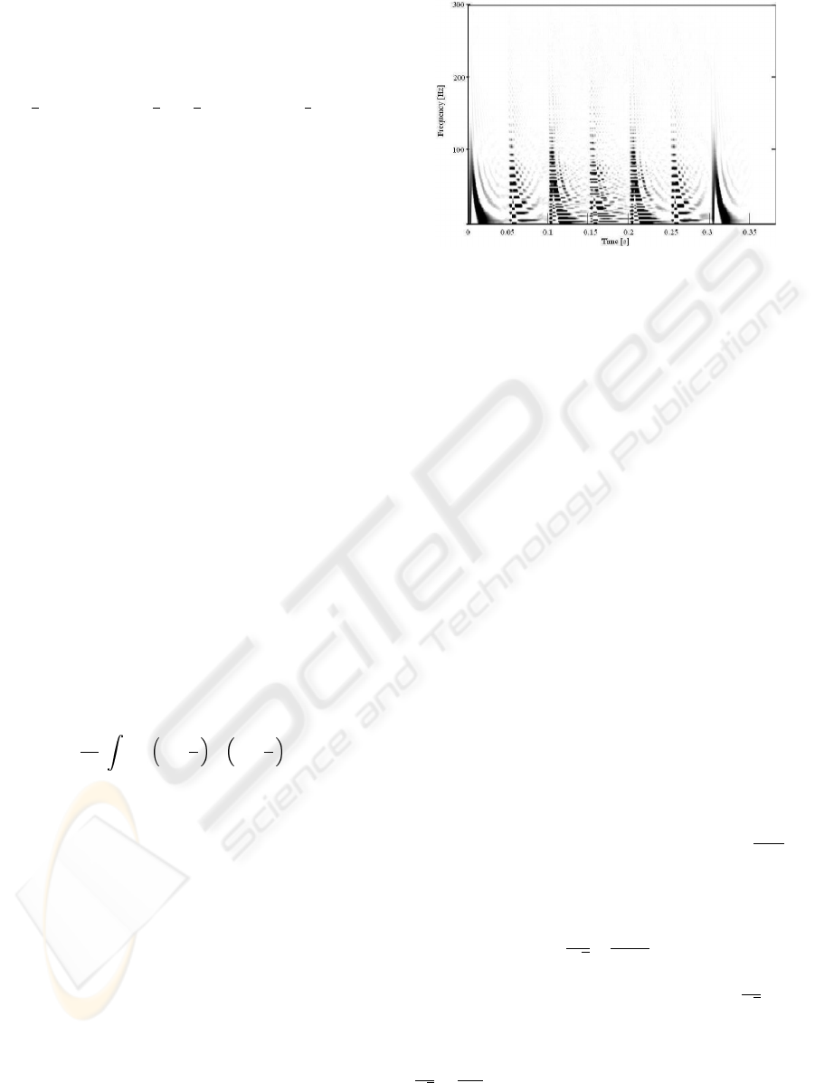
frequency representation may be confusing (see Fig-

ure 2).

Next we show how to eliminate the cross-terms

while maintaining a high-resolution energy distribu-

tion of the servo error.

− P

− Sn

,(2)

(3)

Figure 2: The absolute value of the Wigner distribution of

the servo error signal. Darker means higher relative en-

ergy. Seven intervals can be identiﬁed with signiﬁcant en-

ergy content, of which three spurious ones (2, 4, and 6) due

to cross-terms. Note that also the non-spurious third and

ﬁfth peaks are distorted by cross-terms.

2.2.2 Atomic Decomposition of the Servo Error

and Matching Pursuit in L

(R)

Decomposition of signals over window Fourier trans-

forms and wavelet transforms are the best known ex-

amples of signal decomposition over a family of func-

tions that are well localized in time and frequency. In

this section, we shall discuss time-frequency atomic

decomposition, also known as adaptive decomposi-

tion, of a signal and we shall describe a general it-

erative decomposition algorithm known as matching

pursuit (MP) (Mallat and Zhang, 1993). We shall also

explain why this atomic decomposition is well ﬁtted

for servo error signal decomposition. Based on this

decomposition we shall show the servo error energy

distribution over a simple and complex atomic dictio-

nary.

MP is based on a family D of time-frequency atoms

that can be generated by scaling, translating and mod-

ulating a single window function g ∈ L

(R). We

suppose that the function g is real, continuously dif-

ferentiable, non-zero, g(0) 6= 0 and g(t) ∼ O(

1+t

In addition, we impose that kgk = 1 and that

g(t)dt 6= 0. For any scale s > 0, frequency mod-

ulation φ [Hz] and translation u, one deﬁnes

(t) =

√

t − u

2π jφt

, (5)

with γ = (s, u, φ) ∈ R

× R

. The factor

√

nor-

malizes to 1 the L

norm of g

. We also observe

that atoms deﬁned in (5) look like φ-modulated ver-

sions of a doubly-indexed family of wavelets ψ

s,u

√

ψ(

t−u

), with the difference that for atoms one im-

poses the condition

g(t)dt 6= 0 while the admis-

sibility condition for wavelets requires

ψ(t)dt =

ICINCO 2006 - SIGNAL PROCESSING, SYSTEMS MODELING AND CONTROL

0. If g is even as in most situations, then g

(t) is

well concentrated in time and frequency (Mallat and

Zhang, 1993).

The family D = {g

}

is extremely redundant

(Torresani, 1991). To represent any function h efﬁ-

ciently, we must select an appropriate countable sub-

set of atoms {g

}

so that

h =

∞

n=−∞

. (6)

Consequently, for signals that include scaling and

highly oscillatory structures one cannot deﬁne a priori

appropriate constraints in scale and modulation para-

meters of the atoms g

used in expansion (6). The

elements of the dictionary D = {g

}

need to be

selected adaptively, depending on local properties of

the function h.

In our case, the servo error contains non-stationary

random structures (machine vibrations and sensor

noise), deterministic chaotic vibrations, and subhar-

monic oscillations that are known to demonstrate nar-

row high frequency support (Yen and Lin, 2000).

For this reason, the decomposition of error signals

over triple-indexed time-frequency atoms (5) enables

the extraction of signal features that combine non-

stationary, deterministic chaotic and transient chaotic

characteristics

Next we’ll give an outline of the MP algorithm

in the Hilbert space L

(R). We ﬁrst approximate

h ∈ L

(R) with linear projections on elements of

D. Then it follows that

h =< h, g

> g

+ Rh, (7)

where Rh ∈ L

(R) is the residual after approximat-

ing h in the direction g

. Since g

is orthogonal on

Rh, it follows that

khk

= | < h, g

> |

+ kRhk

To minimize kRhk, we chose g

∈ D such that

| < h, g

> | is maximum. After the ﬁrst step

decomposition (7), we continue iteratively by sub-

decomposing the residual Rh by projecting it on a

vector of D that matches Rh the best, as we have done

for h. Therefore, we inductively obtain the m

order

decomposition of h over the dictionary D,

h =

m−1

n=0

< R

h, g

> g

+ R

h, (8)

where we denote by R

h the residual obtained at the

order decomposition of h. Using (8), one can

easily obtain the following important result:

Theorem.(Mallat and Zhang, 1993) If D is com-

plete (

span(D) = L

(R)) then

h =

∞

n=0

< R

h, g

> g

(9)

and

khk =

∞

n=0

| < R

h, g

> |

. (10)

Remark. Finite linear expansions of time-

frequency atoms (5) are dense in L

(R) and therefore

this dictionary is complete.

The smallest complete dictionaries are bases. By

decomposing a signal onto an orthonormal bases of

compactly supported wavelets having a certain num-

ber of vanishing moments (Daubechies, 1991), cor-

relation between scales is avoided. One-dimensional

well localized in time (compactly supported) wavelets

are of the greatest interest for applications because of

the simplest numerical realization of expansion and

synthesis algorithms. The number of the vanishing

moments is especially important when one wants to

quickly compress large data sets. By using com-

pactly supported wavelets that have a relatively high

number of vanishing moments, the L

norm of the

residual will decrease faster than when using other

wavelets that have less vanishing moments. On the

other hand, for feature extraction tasks, choosing a too

high number of vanishing moments is not desirable as

we are interested in the non-redundant high frequency

components of the signal (Chandroth, 1999). In

other words, we are interested to decompose the sig-

nal into time-frequency atoms that describe the non-

smooth (nonlinear and nonstationary) behavior well

while preserving regular components of the servo er-

ror (Struzik and Siebes, 1998).

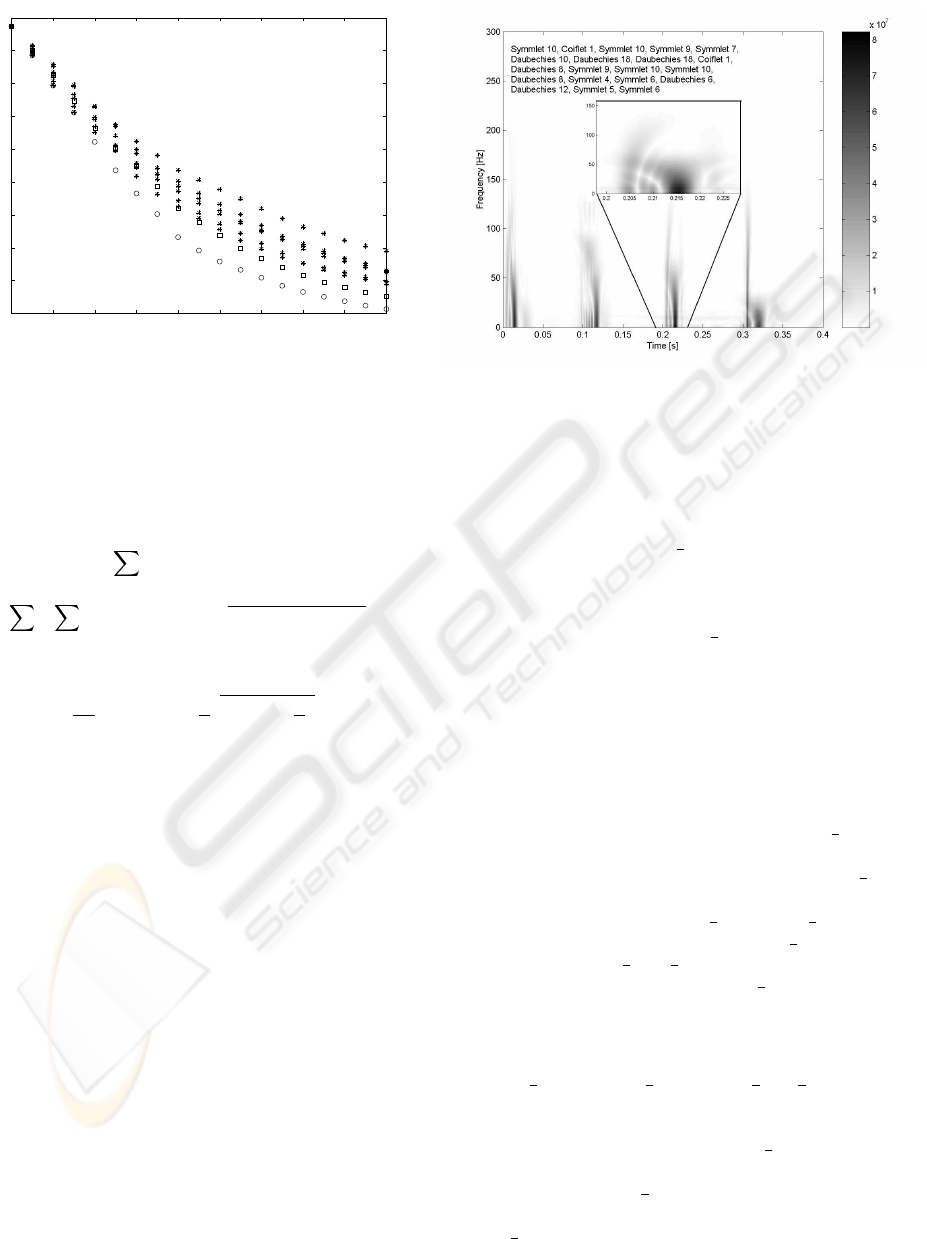
Next we show in Figure 3 the servo error decom-

position with respect to a simple atomic dictionary D

which is built with Symmlets. By applying the MP

algorithm, we found that the decomposition of the

analyzed servo error signal with respect to Symm-

lets with 9 vanishing moments provide the best re-

sults: for a given number of iterations, the L

norm

of the residuals given by formula (8) becomes smaller

than when using other simple atomic dictionaries, like

those that are built with Symmlets {4, 5, 6, 7, 8, 10},

Daubechies, Coiﬂets, and Haar wavelets.

At the end of this section we consider a com-

plex atomic dictionary D built with the asymmet-

ric Daubechies’ wavelets and by their more symmet-

ric and larger supported closely related cousins, i.e.

Symmlets and Coiﬂets (Daubechies, 1991). We ap-

ply the MP algorithm for the servo error decomposi-

tion with respect to this dictionary and we obtain a

smaller L

norm of the residuals (8) than when the

servo error is decomposed with Symmlets, see Fig-

ure 3. Through our numerical experiments we use a

quadrature mirror ﬁlter bank MP algorithm, see (Mal-

lat and Zhang, 1993), (Buckheit et al., 1995), (Rioul

and Vetterli, 1991).

Based on the decomposition (9) of any h ∈ L

(R)

over a simple or complex dictionary, and the deﬁni-

DESIGN OF AN ITERATIVE LEARNING CONTROL FOR A SERVO SYTEM USING MULTI-DICTIONARY

MATCHING PURSUIT

0 2 4 6 8 10 12 14 16 18

0.4

0.6

0.8

1.2

1.4

1.6

1.8

2.2

x 10

Iteration

norm of the residuals

− stars represent decomposition with respect to different members of

the symmlet family 4,5,6,7,8,10 ;

− squares are obtained using symmlets 9 (best of the symmlet family);

− circles are obtained using our dictionary approach

Figure 3: The L

norm of the residuals (8) using a simple

atomic dictionary built with Symmlets. After a relatively

small number of iterations, Symmlets 9 show the best sig-

nal decomposition. The best results, however, are obtained

using our multi-dictionary approach.

tion of the Wigner distribution in (4), we obtain

(t, f ) =

∞

n=0

| < R

h, g

> |

(t, f )+

∞

n=0

∞

m=0,6=n

| < R

h, g

> |

| < R

h, g

> |W

n,m

where

n,m

2π

(t +

)

(t −

−2π jfτ

dτ

denotes the cross Wigner distribution of the atoms g

and g

The double sum corresponds to the cross-terms of

the Wigner distribution that we try to remove in or-

der to obtain a clear time-frequency distribution of

the signal h. We only keep the ﬁrst sum and deﬁne

the energy distribution of the signal h over the time-

frequency plane as

(t, f ) =

∞

n=0

| < R

h, g

> |

(t, f ). (11)

By taking the absolute value of the energy distri-

bution deﬁned in formula (11) with f = e

, when

the dictionary D = {g

} is built with a complex

atomic dictionary generated by Symmlets, Coiﬂets

and Daubechies, we obtain the time-frequency energy

distribution plotted in Figure 4.

2.3 Design of a Bandwidth Proﬁle

Next we shall design a bandwidth proﬁle for the

time-varying robustness ﬁlter introduced in (1).

Figure 4: Servo error energy distribution using a multi-

dictionary wavelet packet generated by combining the

Daubechies, Symmlets and Coiﬂets atoms (selected MP

atoms are listed). The small insert zooms in to show the

’banana’ shapes, i.e. they consist of narrow-band subhar-

monic oscillations and chaotic vibrations.

Consider the time vector

t = (t

)

i∈N

; the initial

feedforward signal u

is chosen identically zero and

the error signal e

is the measured servo error when

a rigid body acceleration feed-forward is applied.

The elements of the vector Ω

(t) are chosen equally

small values, i.e. the initial time-varying robustness

ﬁlter is a steady-state ﬁlter whose bandwidth is

high enough (about 500 [Hz]) such that it does not

ﬁlter the deterministic content of the servo error.

Because of this choice and because the learning ﬁlter

L ∼ P

−1

behaves as a 1000 [Hz] low-pass ﬁlter,

by (2) it follows that the energy distribution of error

signal e

and feedforward signal u

are similar in

shape and for the design of the bandwidth Ω

(

t) it is

not important whether we analyze the servo error e

or its high bandwidth low-pass ﬁltered version u

(

t).

The adaptive update law Ω

(t) → Ω

k+1

(t) for the

design of the time-varying bandwidth Ω

(

t) of the ro-

bustness ﬁlter Q

(s,

t, Ω

(t)) for any iteration k con-

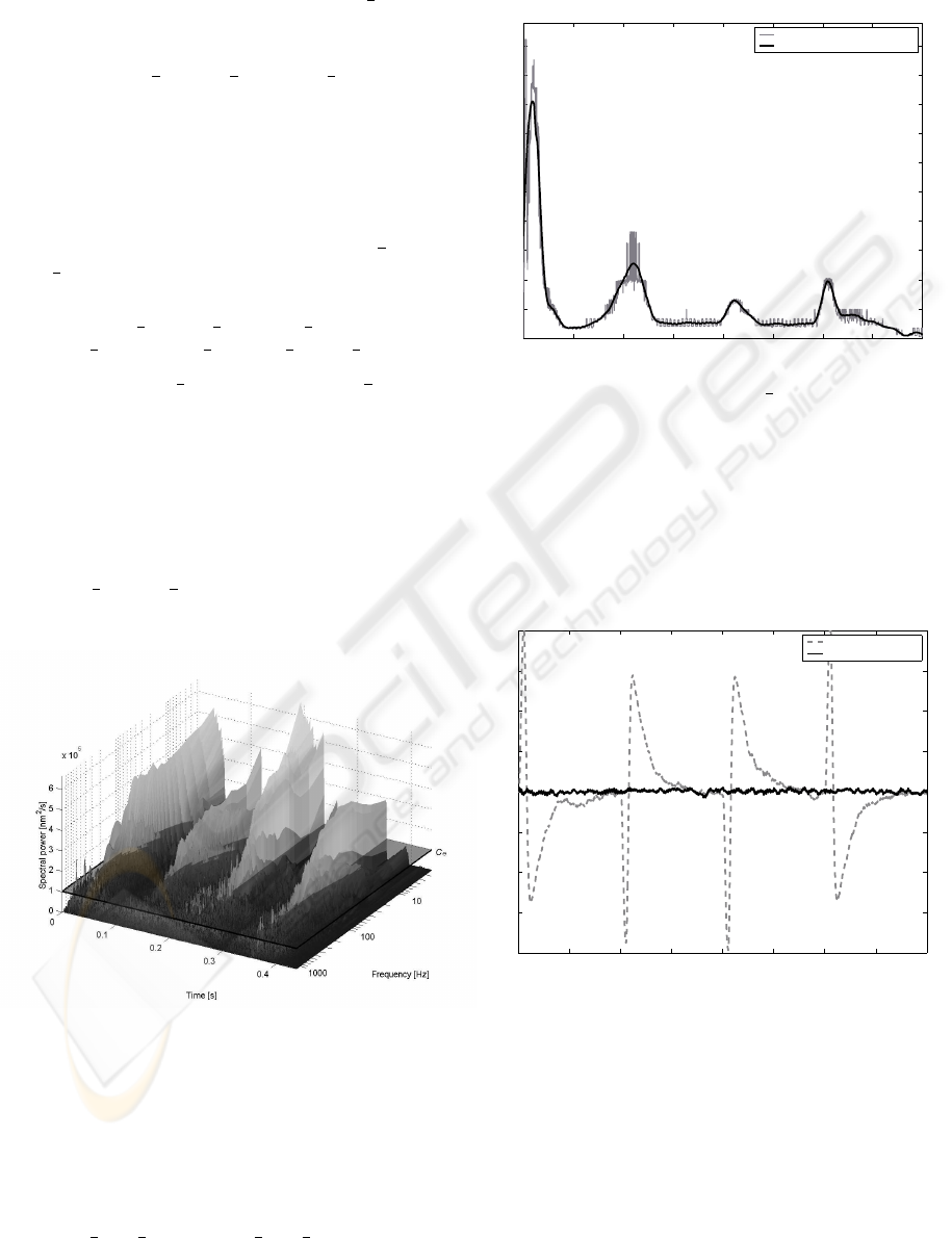
tains the frequency envelope F

max,k

(

t) as gain. This

encompasses the frequencies of all signal components

at each time-instant whose energy exceeds C

, the

value of the noise during standstill:

max,k

(

t) = max(ω

(t)), for H

(t, ω

(t)) ≥ C

(12)

where H

is the time-frequency energy distribu-

tion of the feedforward signal u

, ω

(

t) is the cross-

section of H

and C

height plane (see Figure 5).

The envelope F

max

(t) is used as a gain in an adap-

tive update law. This law changes the bandwidth pro-

ﬁle Ω(t) after each iteration, when the effects of the

ICINCO 2006 - SIGNAL PROCESSING, SYSTEMS MODELING AND CONTROL

previous change on the measured error are evaluated.

After a new bandwidth proﬁle has been implemented,

its beneﬁt is evaluated by the function ∆N

(t), which

compares the local ℓ

norm of the current error to that

of the error at the previous iteration, such that

∆N

(

t) = N

(t) − N

k−1

(t) (13)

where

) =

i+T

j=i−T

), (14)

> 0 gives the width of the window where the sig-

nals are locally compared.

After introducing the terms F

max,k

(

t) and

∆N

(

t), we are now ready now to give the band-

width update rule

Ω

k+1

(

t) = Ω

(t) + ∆Ω

(t),

∆Ω

(

t) = F

max,k

(t) · ∆N

(t) · K

(t)

(15)

where the term K

(

t) = −sign(∆Ω

k−1

(t)) is in-

troduced to add the following logic to the mech-

anism: if the bandwidth was previously increased

(∆Ω

k−1

) > 0), while the error decreased

(∆N

) < 0), this change was beneﬁcial and the

bandwidth may be further increased. On the other

hand, if an increase in the bandwidth resulted in a

larger error, this was obviously not the case and the

bandwidth should be lowered again. The combina-

tion ∆N

(

t) · K

(t) results in this kind of update

behavior.

Figure 5: A 3D-plot of the Wigner distribution for k = 1

(therefore of u

). The horizontal plane at energy value C

discriminates deterministic signal components from noise.

As the learning ﬁlter L ∼ P

−1

behaves as a 1000 [Hz]

low-pass ﬁlter, by (2) and (3) it follows that the energy dis-

tribution of error signal e

and feedforward signal u

are

similar in shape.

Applying the above algorithm in this section

with H

(

t, ω

(t))

def

≡ E

(t, ω

(t)) to the multi-

dictionary approach, we obtain he bandwidth proﬁle

plot in Figure 6.

0 0.05 0.1 0.15 0.2 0.25 0.3 0.35 0.4

100

150

200

250

300

350

400

450

500

Time [s]

Ω[Hz]

The bandwidth Ω

The smoothed approximation of Ω

Figure 6: The bandwidth proﬁle Ω(t) at iteration k = 1;

design based on the servo error energy distribution over the

complex time-frequency atomic dictionary found in the end

of Section 2.2.

Finally, in Figure 7 we show the servo error signal

when Adaptive ILC with the bandwidth of the Q-ﬁlter

as shown in Figure 6 is implemented on the wafer

stage test rig.

0 0.05 0.1 0.15 0.2 0.25 0.3 0.35 0.4

−4

−3

−2

−1

x 10

−7

Time [s]

Servo error [m]

using acceleration FF

using ILC, 3

iteration

Figure 7: Error signal when rigid body accleration feedfor-

ward is applied and Adaptive ILC with the bandwidth of the

Q-ﬁlter as shown in Figure 6.

3 CONCLUSIONS

When comparing the resulting time-frequency energy

distributions in Figures 2 and 4, we note the follow-

ing:

DESIGN OF AN ITERATIVE LEARNING CONTROL FOR A SERVO SYTEM USING MULTI-DICTIONARY

MATCHING PURSUIT

The energy distribution based on the complex

atomic dictionary in Figure 4 is better localized in

time and frequency than the other. Also its resolu-

tion is much higher, and its high-energy deterministic

components can be much better separated from low-

energy stochastic components.

As we have announced, we are not only interested

in separating deterministic and stochastic components

in control signals, but also in separating their con-

stituents, i.e. periodic, subharmonic, chaotic and tran-

sient for deterministic nonlinear time-varying com-

ponents versus non-stationary and stationary for sto-

chastic components. The non-stationary and deter-

ministic chaotic vibrations present in the servo error

signal have narrow high-frequency support and are

difﬁcult to be detected using Wigner distribution. By

applying the adaptive decomposition algorithm de-

scribed in Section 2.2.2, we are also able to identify

such narrow-band frequency characteristics, as can be

seen from the ‘banana’ shape of the dark patterns in

Figure 4, which are much more expressive than the

black patterns in Figure 2.

In Figure 2 the local cross-terms around t =

{0, 0.1, 0.2, 0.3} are not eliminated, while in Figure

4 they are not present anymore.

The energy plot in Figure 4 does not contain cross-

terms and any numerically undesired effects, as in

Figure 2.

Additionally, our multi-dictionary approach leads

to a clearer identiﬁcation of time-varying non-linear

and stochastic servo error components and therefore,

to an improved adaptive ILC design.

We further observe that an overall smaller band-

width than in Figure 2 is obtained (not higher than

about 400 [Hz] in the beginning of the acceleration

proﬁle and 100 [Hz] around other jerk moments).

Therefore, the ILC needs to learn only around these

jerk moments up to smaller frequencies than those

found when Wigner distribution was applied for the

computation of the bandwidth proﬁle.

This means that the stochastic effects will not be

ampliﬁed unnecessarily (high bandwidth means good

tracking performance and noise ampliﬁcation) while

all existent deterministic effects will be learned. Also,

unlike in Figure 2, we do not obtain any increased

bandwidth because of cross terms: the bandwidth of

the Q-ﬁlter needs to be increased just around the jerk

moments while, in between, a small bandwidth can be

maintained.

Also, as seen in Figure 4, the bandwidth proﬁle has

a very good smooth approximation. Therefore, fast

switching between the cut-off frequency of Q-ﬁlters

that corresponds to different time instances is avoided

and the stability of the switched ILC system is not an

issue anymore.

REFERENCES

Buckheit, J., Chen, S., Donoho, D., Johnstone, I., and Scar-

gle, J. (1995). Wavelab. In Tech. Rep., Stanford Uni-

versity.

Cappellini, V. and Constantinides, A. (1984). Interference

terms in the Wigner distribution. Digital Signal Proc.

Casalino, G. and Bartolini, G. (1984). A learning proce-

dure for the control of movements of robotic manipu-

lators. In Proc. 4th IASTED Symp. Robotics Automa-

tion, pages 108–111.

Chandroth, G. O. (1999). Diagnostic classiﬁer ensembles:

Enforcing diversity for reliability in the combination.

In University of Shefﬁeld, UK.

Chang, C.-K., Longman, R. W., and Phan, M. Q. (1992).

Techniques for improving transients in learning con-

trol systems. Adv. Astronautic. Sci, 76:20352052.

Chen, Y. and Moore, K. (2001). Frequency domain adap-

tive learning feedforward control. In Proc. of the 2001

IEEE Int. Symp. Comp. Intell. Robotics and Automa-

tion, pages 396–401.

Cohen, L. (1989). Time-frequency distributions – a review.

Proc. IEEE, 77(7).

Daubechies, I. (1991). Ten lectures on wavelets. Series in

Applied mathematics, SIAM.

Goh, C. J. (1994). A frequency domain analysis of learn-

ing control. J. Dynamic Syst., Measurement, Contr.,

116:781–786.

Mallat, S. and Zhang, Z. (1993). Matching pursuit with

time-frequency dictionaries. IEEE Trans. on Signal

Processing, 41(12):3397–3415.

Margrave, G. F. (1998). Theory of nonstationary linear ﬁl-

tering in the fourier domain with applications to time-

variant ﬁltering. Geophysics, 63(1):244 – 259.

Mecklenbr

auker, W., Hlawatsch, F., and Janssen, A. (1997).

The wigner distribution, theory and applications in

signal processing. Elsevier.

Moore, K. L. (1993). Iterative learning control for de-

terministic systems. Adv. in Ind. Control. Springer-

Verlag.

Norrl

of, M. (2002). Iteration varying ﬁlters in iterative

learning control. In Proc. 4th Asian Control Conf.,

page 21242129.

Rioul, O. and Vetterli, M. (1991). Wavelets and sig-

nal processing. IEEE Signal Processing Magazine,

8(4):14–38.

Rotariu, I., Dijkstra, B., and Steinbuch, M. (2004). Com-

parison of standard and lifted ilc on a motion system.

In 3rd IFAC Symp. Mechatronic Systems, Sydney, Aus-

tralia, pages 211–6.

Rotariu, I., Ellenbroek, R., and Steinbuch, M. (2003a).

Time-frequency analysis of a motion system with

learning control. In Proc. ACC Conf., pages 3650 –

3654. American Control Conf.

ICINCO 2006 - SIGNAL PROCESSING, SYSTEMS MODELING AND CONTROL

Rotariu, I., Ellenbroek, R., and Steinbuch, M. (2006).

Adaptive iterative learning control with application to

a wafer stage. submitted to IEEE Transactions on

Control Systems Technology.

Rotariu, I., Ellenbroek, R., van Baars, G., and Steinbuch, M.

(2003b). Scan-length independent iterative learning

control applied to a wafer stage motion system. In

Proc. ECC Conf.

Struzik, Z. and Siebes, A. (1998). Wavelet transform in sim-

ilarity paradigm i and ii. In Centrum voor Wiskunde

en Informatica, Report,INS-R9802.

Tang, X., Cai, L., and Huang, W. (2000). A learning

controller for robot manipulators using fourier series.

IEEE Trans. Robot. Automat., 16(1):3645.

Tharayil, M. and Alleyne, A. (2004). Design and conver-

gence of a time-varying iterative learning control law.

In Proc. IMECE Int. Mech. Eng. Congr. and R&D

Expo.

Torresani, B. (1991). Wavelets associated with represen-

tations of the aﬁne weyl-heisenberg group. J. Math

Physics, 32(5):1273–9.

Wirkander, S.-L. and Longman, R. (1999). Limit cycles for

improved performance in self-tuning learning control.

Adv. Astronautic. Sci., 102:763–781.

Yen, G. and Lin, K. (2000). Wavelet packet feature ex-

traction for vibration monitoring. IEEE Trans. Ind.

Electronics, 47(3):650–67.

Zhang, B., Wang, D., and Ye, Y. (2005). Wavelet transform-

based frequency tuning ilc. IEEE Trans. Systems, Man

& Cybernetics, Part B: Cybernetics, 35(1):107–114.

Zheng, D. and Alleyne, A. (2001). Adaptive iterative

learning control for systems with non-smooth non-

linearities. In Proc. ASME Conf., Pittsburgh, Penn-

sylvania. ASME Int. DETC.

Zheng, D. and Alleyne, A. (2003). Stability of a novel iter-

ative learning control scheme with adaptive ﬁltering.

In Proc. ACC Conf.

DESIGN OF AN ITERATIVE LEARNING CONTROL FOR A SERVO SYTEM USING MULTI-DICTIONARY

MATCHING PURSUIT