
SIMULTANEOUS LOCALIZATION AND MAPPING IN
UNMODIFIED ENVIRONMENTS USING STEREO VISION
A. Gil, O. Reinoso, C. Fern
´
andez, M. A. Vicente
Universidad Miguel Hern
´
andez de Elche
Avda. de la Universidad s/n, 03202 Elche (Alicante)
A. Rottmann, O. Mart
´
ınez Mozos
University of Freiburg
Department of Computer Science
D-79110 Freiburg
Keywords:
SLAM, Stereo Vision, Visual landmarks, Data Association.
Abstract:
In this paper we describe an approach that builds three dimensional maps using visual landmarks extracted
from images of an unmodified environment. We propose a solution to the Simultaneous Localization and
Mapping (SLAM) problem for autonomous mobile robots using visual landmarks. Our map is represented
by a set of three dimensional landmarks referred to a global reference frame, each landmark contains a visual
descriptor that partially differentiates it from others. Significant points extracted from stereo images are used
as natural landmarks, in particular we employ SIFT features found in the environment. We estimate both
the map and the path of the robot using a Rao-Blackwellized particle filter, thus the problem is decomposed
into two parts: one estimation over robot paths using a particle filter, and N independent estimations over
landmark positions, each one conditioned on the path estimate. We actively track visual landmarks at a local
neighbourhood and select only those that are more stable. When a visual feature has been observed from a
significant number of frames it is then integrated in the filter. By this procedure, the total number of landmarks
in the map is reduced, compared to prior approaches. Due to the tracking of each landmark, we obtain different
examples that represent the same natural landmark. We use this fact to improve data association. Finally,
efficient resampling techniques have been applied, which reduces the number of particles needed and avoids
the particle depletion problem.
1 INTRODUCTION
Building an accurate map of a given environment is
one of the hardest tasks for a mobile robot. It is inher-
ently difficult, since noise in the estimation of robot’s
pose leads to errors in the estimation of the map and
vice-versa. Recently, many authors have considered
the problem of Simultaneous Localization and Map-
ping (SLAM). The aim of SLAM is to build a map of
an unknown environment and simultaneously localise
the robot with respect to this map. Here we consider
this problem using a Rao-Blackwellized Particle Fil-
ter (RBPF).
Most work on SLAM so far has focussed on build-
ing 2D maps of environments using range sensors
such as SONAR and laser (Wijk and Christensen,
2000), (Thrun, 2001). Recently, Rao-Blackwellized
particle filters have been used as an effective mean
of solving the SLAM problem using occupancy grid
maps (Stachniss et al., 2004). In this approach, each
particle constructs its own map based on the obser-
vations and the trajectory for that particle. Parti-
cles which best explain current observations are given
higher weights and re-sampled.
While mapping a particular environment, one must
be aware of two key problems:
• Odometry is subject to cumulative drift.
• Landmarks can be ambiguous.
Recently, some authors have been concentrating on
building three dimensional maps using visual infor-
mation extracted from cameras. In this scenario, the
map is represented by a set of three dimensional land-
marks related to a global reference frame. Stereo sys-
tems are typically less expensive than laser sensors
and are able to provide directly 3D information from
the scene. In (Little et al., 2001) and (Little et al.,
2002) stereo vision is used to track 3D visual land-
marks extracted from the environment. In this work,
SIFT features are used as visual landmarks. SIFT
(Scale Invariant Feature Transform) where initially
invented by D. Lowe and used in object recognition
tasks (Lowe, 1999). During exploration, the robot
extracts SIFT features from stereo images and calcu-
302
Gil A., Reinoso O., Fernández C., A. Vicente M., Rottmann A. and Martínez Mozos O. (2006).
SIMULTANEOUS LOCALIZATION AND MAPPING IN UNMODIFIED ENVIRONMENTS USING STEREO VISION.
In Proceedings of the Third International Conference on Informatics in Control, Automation and Robotics, pages 302-309
DOI: 10.5220/0001207303020309
Copyright
c
SciTePress

lates relative measurements to them. Landmarks are
then integrated in the map with an Extended Kalman
Filter associated to it. However, this approach does
not manage correctly the uncertainty associated with
robot motion, and only one hypothesis over the pose
of the robot is maintained. Consequently it may fail
in the presence of large odometric errors (e.g. while
closing a loop). In (Mir
´
o et al., 2005) a Kalman fil-
ter is used to estimate an augmented state constituted
by the robot pose and N landmark positions (Dis-
sanayake et al., 2001). SIFT features are used too
to manage the data association among visual land-
marks. However, since only one hypothesis is main-
tained over the robot pose, the method would fail in
the presence of incorrect data associations. In addi-
tion, in the presence of a significant number of land-
marks the method would be computationally expen-
sive.
The work presented in (Sim et al., 2005) uses SIFT
features as significant points in space and tracks them
over time. It uses a Rao-Blackwellized particle filter
to estimate both the map and the path of the robot.
The robot movement is here estimated from stereo
ego-motion (Little et al., 2001), providing a corrected
odometry that simplifies the SLAM problem, since no
large odometric errors are introduced.
The most relevant contribution of this paper is
twofold. First, we present a new mechanism to deal
with the data association problem in the case of dif-
ferent landmarks with similar appearance. This fact
may occur in most environments. Second, our ap-
proach actively tracks landmarks prior to its integra-
tion in the map. As a result only those landmarks
that are more stable are incorporated in the map. By
using this approach, our map typically consists of a
reduced number of landmarks compared to those of
(Little et al., 2002) and (Sim et al., 2005), for compa-
rable map sizes. In addition, we have applied effec-
tive resampling techniques, as exposed in (Stachniss
et al., 2005). This fact reduces the number of particles
needed to construct the map, thus reducing computa-
tional time.
The remainder of the paper is structured as follows.
Section 2 deals with visual landmarks and their utility
in SLAM. Section 3 explains the basics of the Rao-
Blackwellized particle filter. Next, section 4 presents
our solution to the data association problem in the
context of visual landmarks. In section 5 we present
our experimental results. Finally, section 6 sums up
the most important conclusions and proposes future
extensions.
2 FEATURE-BASED METHODS:
VISUAL FEATURES
Previous works in map building has revolved around
two topics: occupancy or certainty grids, and feature-
based methods. Feature based methods work by lo-
cating features in the environment, estimating their
position, and then using them as known landmarks.
Different kinds of features have been used to create a
map of the environment. In our work, we use visual
landmarks as features to build the map. In particular,
we use SIFT features (Scale Invariant Feature Trans-
form) which were developed for image feature gen-
eration, and used initially in object recognition ap-
plications (see (Lowe, 2004) and (Lowe, 1999) for
some examples). Key locations are selected at max-
ima and minima of a difference of Gaussian function
applied in scale space. The features are invariant to
image translation, scaling, rotation, and partially in-
variant to illumination changes and affine or 3D pro-
jection. They are computed by building an image
pyramid with resampling between each level. SIFT
locations extracted by this procedure may be under-
stood as significant points in space that are highly dis-
tinctive, thus can be found from a set of robot poses.
In addition, each SIFT location is given a descriptor
that describes this landmark. Thus, this process en-
ables the same points in the space to be recognized
from different viewpoints, which may occur while
the robot moves around its workplace, thus providing
information for the localization process. SIFT fea-
tures have been used in robotic applications, showing
its suitability for localization and SLAM tasks (Little
et al., 2001), (Little et al., 2002), (Sim et al., 2005).
Figure 1 shows a visual features extracted from an im-
age. These SIFT locations are used as landmarks in
the map. The size of the arrow on each feature is pro-
portional to SIFT’s scale.
3 RAO-BLACKWELLIZED SLAM
We estimate the map and the path of the robot using
a Rao-Blackwellized particle filter. Using the nomen-
clature in this filter, we denote as s
t
the robot pose at
time t. On the other hand, the robot path until time
t will be denoted s
t
= {s
1
, s
2
, . . . , s
t
}, the set of
observations made by the robot until time t will be
denoted z
t
= {z
1
, z
2
, . . . , z
t
} and the set of actions
u
t
= {u
1
, u
2
, . . . , u
t
}. Therefore, the SLAM prob-
lem can be formulated as that of determining the lo-
cation of all landmarks in the map Θ and robot poses
s
t
from a set of measurements z
t
and robot actions
u
t
. The map is composed as a set of differente land-
marks Θ = {θ
1
, θ
2
, . . . θ
i
, . . . , θ
N
}. We call c
t
to
the correspondence of the landmarks extracted from
SIMULTANEOUS LOCALIZATION AND MAPPING IN UNMODIFIED ENVIRONMENTS USING STEREO VISION
303
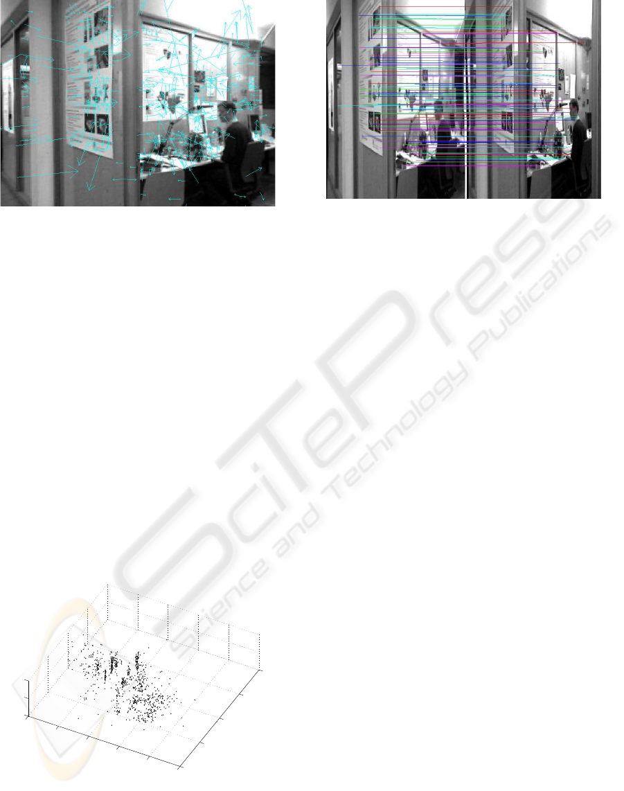
Figure 1: Image shows SIFT locations extracted from a typ-
ical image. The size of the arrow is proportional to SIFT’s
scale.
the data association problem. In consequence, the
SLAM problem can be formulated as the estimation
of the following probability density function over ro-
bot poses:
p(s
t
, Θ|z
t
, u
t
, c
t
) (1)
The map Θ is represented by a collection of N
landmarks. Each landmark is described as: θ
k
=
{µ
k
, Σ
k
, d
k
}, where µ
k
= (X
g
k
, Y
g
k
, Z
g
k
) is a vector
describing the position of the landmark referred to a
global reference frame O
g
with associated covariance
matriz Σ
k
. In addition, each landmark θ
k
is associ-
ated with a SIFT descriptor d
k
that partially differen-
tiates it from others. This map representation is com-
pact and has been used to effectively localize a robot
in unmodified environments (Gil et al., 2005). We can
see in figure 2 an example of the map represented by
N landmarks in a section of the environment.
−10
0
10
20
30
−15
−10
−5
0
5
10
0
1
2
X (m)
Y (m)
Z (m)
Figure 2: Example of the map created by a set of N 3D land-
marks in a section of the environment in which the robot is
present.
While exploring a particular environment, the robot
Figure 3: Stereo correspondences using SIFT features. The
epipolar constrain is used to find correspondences across
images.
needs to determine whether a particular observation
z
t,k
corresponds to a previously mapped landmark or
to a new one. For the moment, we consider this cor-
respondence as known. Given that, at a time t the
map is formed by N landmarks, the correspondence
is represented by c
t
= {c
t,1
, c
t,2
, . . . , c
t,B
}, where
c
t,i
∈ [1 . . . N]. In consequence at a time t the ob-
servation z
t,k
corresponds to the landmark c
t,k
in the
map. When no correspondence is found we denote it
as c
t,i
= N + 1, indicating that it is a new landmark.
3.1 Stereo SIFT
Given two images I
L
t
and I
R
t
, captured with a stereo
head at a time t, we extract natural landmarks which
correspond to points in the 3-dimensional space. Each
point is accompanied by its SIFT descriptor and then
matched across images. The matching procedure is
constrained by the well-known epipolar geometry of
the stereo rig. In addition, a comparison between
SIFT descriptors is used to avoid false correspon-
dences. As a result, at a time t we obtain a set of B
observations denoted by z
t
= {z
t,1
, z
t,2
, . . . , z
t,B
} =
{v
t,1
, d
t,1
, v
t,2
, d
t,2
, . . . , v
t,B
, d
t,B
}. A particular ob-
servation is constituted by z
t,k
= (v
t,k
, d
t,k
), where
v
t,k
= (X
r
, Y
r
, Z
r
) is a three dimensional vector
represented in the left camera reference frame and
d
t,k
is the SIFT descriptor associated to that point.
Figure 3 shows two stereo images of the environ-
ment. Correspondences found across both images are
shown. After stereo correspondence, a 3D reconstruc-
tion of the points is obtained, obtaining B measure-
ments v
t,k
= (X
r
, Y
r
, Z
r
) relative to the left camera
reference frame.
ICINCO 2006 - ROBOTICS AND AUTOMATION
304

3.2 Particle Filter Estimation
The conditional independence property of the SLAM
problem implies that the posterior (1) can be factored
as (Montemerlo et al., 2002):
p(s
t
, Θ|z
t
, u
t
, c
t
) = p(s
t
|z
t
, u
t
, c
t
)
N
k=1
p(θ
k
|s
t
, z
t
, u
t
, c
t
)
(2)
This equation states that the full SLAM posterior is
decomposed into two parts: one estimator over robot
paths, and N independent estimators over landmark
positions, each conditioned on the path estimate. This
factorization was first presented by Murphy in 1999
(Murphy, 1999). We approximate p(s
t
|z
t
, u
t
, c
t
) us-
ing a set of M particles, each particle having N inde-
pendent landmark estimators (implemented as EKFs),
one for each landmark in the map. Each particle is
thus defined as:
S
[m]
t
= {s
t,[m]
, µ
[m]
t,1
, Σ
[m]
t,1
, . . . , µ
[m]
t,N
, Σ
[m]
t,N
} (3)
Where µ
[m]
t,i
is the best estimation at time t for the
position of landmark θ
i
based on the path of the parti-
cle m and Σ
[m]
t,i
its associated covariance matrix. The
particle set S
t
= {S
[1]
t
, S
[2]
t
, . . . , S
[M]
t
, } is calculated
incrementally from the set S
t−1
at time t − 1 and the
robot control u
t
. Thus, each particle is sampled from
a proposal distribution s
[m]
t
∼ p(s
t
|s
t−1
, u
t
). Next,
and following the approach of (Montemerlo et al.,
2002) each particle is then assigned a weight accord-
ing to:
ω
[m]
t,i
=
1
p
|2πZ
c
t,i
|
exp{−
1
2
a} (4)
where
a = (v
t,i
− ˆv
t,c
t,i
)
T
[Z
c
t,i
]
−1
(v
t,i
− ˆv
t,c
t,i
)
Where v
t,i
is the current measurement and ˆv
t,c
t,i
is the predicted measurement for the landmark c
t,i
based on the pose s
[i]
t
. The matrix Z
c
t,i
is the co-
variance matrix associated with the innovation (v
t,i
−
ˆv
t,c
t,i
). Note that we implicitly assume that each mea-
surement v
t,i
has been assigned to the landmark c
t,i
of the map. This problem is, in general, hard to solve,
since similar-looking landmarks may exist. In section
4 we describe our approach to this problem. In the
case that B observations from different landmarks ex-
ist at a time t, we calculate the total weight assigned
to the particle as:
ω
[m]
t
=
B
Y
i=1
w
[m]
t,i
(5)
3.3 Efficient Resampling
In order to assess for the difference between the
proposal and the target distribution, each particle is
drawn with replacement with probability proportional
to this importance weight. During resampling, parti-
cles with a low weight are normally replaced by oth-
ers with a higher weight. It is a well known prob-
lem that the resampling step may delete good particles
from the set and cause particle depletion. In order to
avoid this problem we follow an approach similar to
(Stachniss et al., 2004). Thus we calculate the number
of efficient particles N
eff
as:
N
eff
=
1
P
M
i=1
ω
[i]
t
(6)
We resample each time N
eff
drops below a prede-
fined threshold (set to M/2 in our application). By
using this approach we have verified that the number
of particles needed to achieve good results is reduced.
4 DATA ASSOCIATION
While the robot explores the environment it must de-
cide whether the observation z
t,k
= (v
t,k
, d
t,k
) corre-
sponds to a previously mapped landmark or to a dif-
ferent landmark. We use each associated SIFT de-
scriptor d
t,k
to improve the data association process.
Each SIFT descriptor is a 128-long vector computed
from the image gradient at a local neighbourhood
of the interest point. Experimental results in object
recognition applications have showed that this de-
scription is robust against changes in scale, viewpoint
and illumination (Lowe, 2004). In the approaches
of (Little et al., 2001), (Little et al., 2002) and (Sim
et al., 2005), data association is based on the squared
Euclidean distance between descriptors. In conse-
quence, given two SIFT descriptors d
i
and d
j
the fol-
lowing distance function is computed:
E = (d
i
− d
j
)(d
i
− d
j
)
T
(7)
Then, the landmark of the map that minimizes the
distance E is chosen. Whenever the distance E is be-
low a certain threshold, the two landmarks are con-
sidered to be the same. On the other hand, a new
landmark is created whenever the distance E exceeds
a pre-defined threshold. When the same point is
viewed from slightly different viewpoints and dis-
tances, the values in its SIFT descriptor remain almost
unchanged. However, when the same point is viewed
from significantly different viewpoints (e.g. 30 de-
grees apart) the difference in the descriptor is remark-
able. In the presence of similar looking landmarks,
SIMULTANEOUS LOCALIZATION AND MAPPING IN UNMODIFIED ENVIRONMENTS USING STEREO VISION
305
(a) (b) (c)
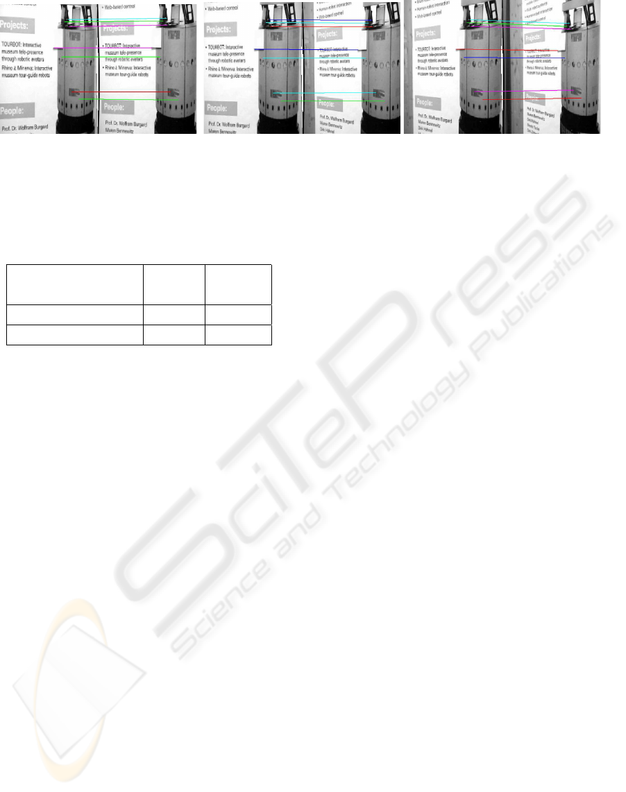
Figure 4: Figures (a)-(c) show different SIFT points tracked along different images with variations in scale and orientation.
Table 1: Comparison of correct and incorrect matches using
the Euclidean distance and the Mahalanobis distance.
Correct Incorrect
matches matches
Euclidean distance 83.85 16.15
Mahalanobis distance 94.04 5.96
this fact causes a significant number of false corre-
spondences, as can be seen in the first column of table
1.
We propose a different method to deal with the data
association in the context of SIFT features. We ad-
dress the problem from a pattern classification point
of view. We consider the problem of assigning a pat-
tern d
j
to a class C
i
. Each class C
i
models a land-
mark. We consider different views of the same vi-
sual landmark as different patterns belonging to C
i
.
Whenever a landmark is found, it is tracked along p
frames and its descriptors d
1
, d
2
, . . . , d
p
are stored.
Then, for each landmark C
i
we compute a mean value
¯
d
i
and estimate a covariance matrix S
i
, assuming the
elements in the SIFT descriptor independent. Based
on this data we compute the Mahalanobis distance:
L = (
¯
d
i
−
¯
d
j
)S
−1
i
(
¯
d
i
−
¯
d
j
)
T
(8)
Where S
i
is a diagonal covariance matrix associ-
ated with the class C
i
with mean value
¯
d
i
. We com-
pute the distance L for all the landmarks in the map
of each particle and assign the correspondence to the
landmark that minimizes L. If none of the values ex-
ceeds a predefined threshold then we consider it a new
landmark.
In order to test this distance function we have
recorded a set of images with little variations of view-
point and distance (see figure 4). SIFT landmarks
are easily tracked across consecutive frames, since the
variance in the descriptor is low. In addition, we visu-
ally judged the correspondence across images. Based
on these data we compute the matrix S
i
for each SIFT
point tracked for more than 5 frames. Following, we
compute the distance to the same class using equa-
tion (7) and (8). For each experiment, we select the
class that minimises its distance function and as we
already know the correspondences, we can compute
the number of mistakes and correct matches. Table 1
shows the results based on our experiments. A total
of 3000 examples where used. As can be clearly seen,
a raw comparison of two SIFT descriptors using the
Euclidean distance does not provide total separation
between landmarks, since the descriptor can vary sig-
nificantly from different viewpoints. As can be seen,
the number of false correspondences is reduced by us-
ing the Mahalanobis distance.
By viewing different examples of the same land-
mark we are able to build a more complete model
of it and this permits us to better separate each land-
mark from others. We consider that this approach re-
duces the number of false correspondences and, con-
sequently produces better results in the estimation of
the map and the path of the robot, as will be shown in
section 5.
5 EXPERIMENTAL RESULTS
During the experiments we used a B21r robot
equipped with a stereo head and a LMS laser range
finder. We manually steered the robot and moved
it through the rooms of the building 79 of the Uni-
versity of Freiburg. A total of 507 stereo im-
ages at a resolution of 320x240 were collected.
The total traversed distance of the robot is ap-
proximately 80m. For each pair of stereo im-
ages a number of correspondences were established
and observations z
t
= {z
t,1
, z
t,2
, . . . , z
t,B
} =
{v
t,1
, d
t,1
, v
t,2
, d
t,2
, . . . , v
t,B
, d
t,B
} were obtained.
After stereo correspondence, each point is tracked for
a number of frames. By this procedure we can assure
that the SIFT point is stable and can be viewed from a
significant number of robot poses. Practically, when a
landmark has been tracked for more than 5 frames it is
ICINCO 2006 - ROBOTICS AND AUTOMATION
306
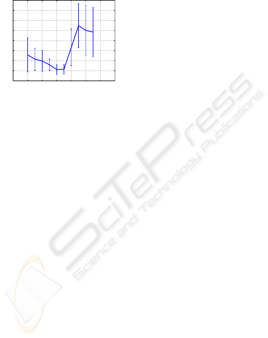
0 0.1 0.2 0.3 0.4 0.5 0.6 0.7
0.2
0.4
0.6
0.8
1
1.2
1.4
1.6
1.8
p
0
RMS position error (m)
Figure 5: Results in RMS localization error when varying
p
0
.
considered a new observation and is integrated in the
filter. As mentioned in section 4, each descriptor is
now represented by d
t,i
= {
¯
d
t,i
, S
i
} where
¯
d
t,i
is the
SIFT vector computed as the mean of the p tracked
landmarks and S
i
is the corresponding diagonal co-
variance matrix.
5.1 Threshold Selection
In a practical way, given a SIFT descriptor and a pre-
dicted landmark position, the robot needs to decide
wether a particular observation belongs to a landmark
c
t,k
in the map or it is a new one. In our approach we
used equation 8 and set up a particular threshold p
0
.
Based on a particular observation z
t,k
= {v
t,k
, d
t,k
,
we find the landmark that minimizes L for the land-
marks that lay in a neighbourhood. When the distance
L exceeds p
0
for all the landmarks in the neighbour-
hood, we create a new landmark. If L < p
0
for a
particular landmark in the map, we update its Kalman
filter. In consequence if p
0
is set too low, landmarks
will be frequently confused. On the contrary, if we
set p
0
too high, new landmarks will be frequently cre-
ated, which affects the quality of the estimated path
and the resulting map.
To test the influence of p
0
we repeatedly ran the al-
gorithm changing its value. Figure 5 shows the RMS
error in the position of the robot when the value of p
0
is changed. In order to test the quality of our results,
we have compared the estimated pose of our method
with the estimated pose using laser data recorded
during exploration. To calculate the pose based on
laser measurements, the method exposed in (Stach-
niss et al., 2004) was used. The SLAM algorithm
was run several times for each value of p
0
. Finally,
to build the map we choose the value of p
0
that pro-
duces better results. During SLAM, the true pose of
the robot is not known, in consequence, the value of
p
0
that produces better results cannot be calculated by
this way. However, we believe that the chosen value
of p
0
will produce good results when mapping differ-
ent environments.
Figure 6 shows the map constructed with 1, 10, and
100 particles. A total number of 1500 landmarks were
estimated. It can be seen that, with only 10 parti-
cles, the map is topologically correct. As can be seen
in the figures, some areas of the map do not possess
any landmark. This is due to the existence of feature-
less areas in the environment (i.e. texture-less walls),
where no SIFT features can be found.
Figure 7(a) shows the error in localization for each
movement of the robot during exploration using 200
particles. Again, we compare the estimated position
of the robot using our approach to the estimation us-
ing laser data.
In addition, we have compared both approaches
to data association as described in section 4. To do
this, we have made a number of simulations vary-
ing the number of particles used in each simulation.
The process was repeated using both data association
methods. As can be seen in figure 7(b) for the same
number of particles, better localization results are ob-
tained when the Mahalanobis distance is used, thus
improving the quality of the estimated map.
Compared to preceding approaches our method
uses less particles to achieve good results. For ex-
ample, in (Sim et al., 2005), a total of 400 particles
are needed to compute a topologically correct map,
while correct maps have been built using 50 parti-
cles with our method. In addition, our maps typi-
cally consists of about 1500 landmarks, a much more
compact representation than the presented in (Sim
et al., 2005), where the map contains typically around
100.000 landmarks.
6 CONCLUSION AND FUTURE
WORK
In this paper a solution to SLAM based on a Rao-
Blackwellized particle filter has been presented. This
filter uses visual information extracted from cameras.
We have used natural landmarks as features for the
construction of the map. The method is able to build
3D maps of a particular environment using relative
measurements extracted from a stereo pair of cam-
eras.
We have also proposed an alternative method to
deal with the data association problem in the context
of visual landmarks, addressing the problem from a
pattern classification point of view. When different
examples of a particular SIFT descriptor exist (be-
longing to the same landmark) we obtain a proba-
bilistic model for it. Also we have compared the re-
SIMULTANEOUS LOCALIZATION AND MAPPING IN UNMODIFIED ENVIRONMENTS USING STEREO VISION
307
−5 0 5 10 15
−10
−8
−6
−4
−2
0
2
4
6
8
10
X (m)
Y (m)
(a)
−5 0 5 10 15
−10
−8
−6
−4
−2
0
2
4
6
8
10
X (m)
Y (m)
(b)
−5 0 5 10 15
−10
−8
−6
−4
−2
0
2
4
6
8
10
X (m)
Y (m)
(c)
−5 0 5 10 15
−10
−8
−6
−4
−2
0
2
4
6
8
10
X (m)
Y (m)
(d)
Figure 6: Figure 6(a) shows a map created using 1 particle. Figure 6(b) shows a map created using 10 particles and image 6(c)
used 100 particles. We also show superposed the real path (continuous) and the estimated path using our approach (dashed).
Figure 6(d) shows the real path (continuous) and the odometry of the robot (dashed).
sults obtained using the Mahalanobis distance and the
Euclidean distance. By using a Mahalanobis distance
the data association is improved, and, consequently
better results are obtained since most of the false cor-
respondences are avoided.
Opposite to maps created by means of occupancy
or certainty grids, the visual map generated by the ap-
proach presented in this paper does not represent di-
rectly the occupied or free areas of the environment.
In consequence, some areas totally lack of landmarks,
but are not necessary free areas where the robot may
navigate through. For example, featureless areas such
as blank walls provide no information to the robot. In
consequence, the map may be used to effectively lo-
calize the robot, but cannot be directly used for nav-
igation. We believe, that this fact is originated from
the nature of the sensors and it is not a failure of the
proposed approach. Other low-cost sensors such as
SONAR would definitely help the robot in its naviga-
tion tasks.
As a future work we think that it is of particu-
lar interest to further research in exploration tech-
niques when this representation of the world is used.
We would also like to extend the method to the case
where several robots explore an unmodified environ-
ment and construct a visual map of it.
ACKNOWLEDGEMENTS
This research has been supported by a Marie Curie
Host fellowship with contract number HPMT-CT-
2001-00251 and the spanish government (Ministerio
de Educaci
´
on y Ciencia. Projects Ref: DPI2004-
07433-C02-01, and PCT-G54016977-2005). The au-
ICINCO 2006 - ROBOTICS AND AUTOMATION
308
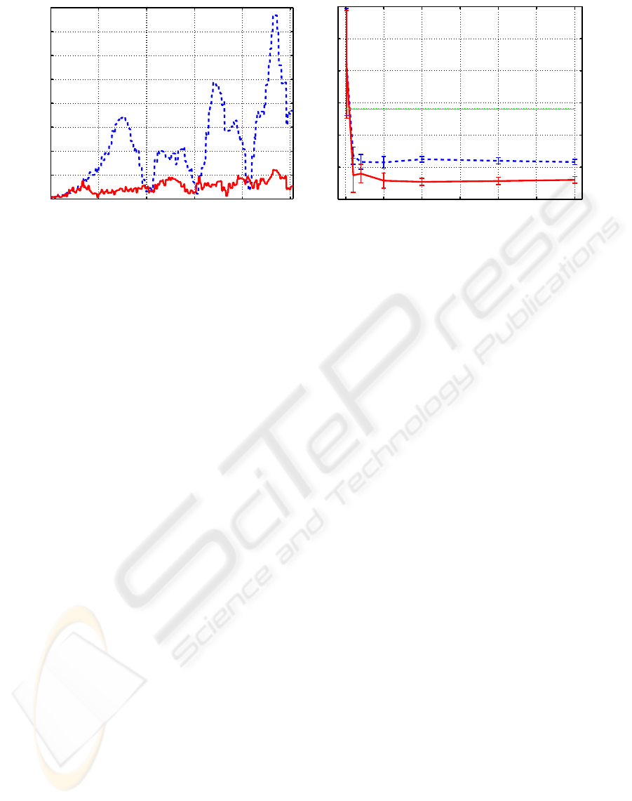
0 100 200 300 400 500
0
0.5
1
1.5
2
2.5
3
3.5
4
Movement number
Position absolute error (m)
(a)
0 50 100 150 200 250 300
0
0.5
1
1.5
2
2.5
3
Number of particles
Position RMS error (m)
(b)
Figure 7: Figure 7(a) shows the absolute position error during the SLAM process. The final error in position is 0.34m. Figure
7(b) shows results in localization error when varying the number M of particles. The RMS error in odometry is shown as a
dotted line. Results using equation (7) are shown as a dashed line and results using equation (8) are shown as a continuous
line.
thors would also like to thank, Rudolph Triebel and
Manuel Mucientes for their help and stimulating dis-
cussions.
REFERENCES
Dissanayake, G., Newman, P., Clark, S., Durrant-Whyte,
H., and Csorba, M. (2001). A solution to the simulta-
neous localization and map building (slam) problem.
IEEE Trans. on Robotics and Automation, 17:229–
241.
Gil, A., Reinoso, O., Vicente, A., Fern
´
andez, C., and Pay
´
a,
L. (2005). Monte carlo localization using sift fea-
tures. Lecture Notes in Computer Science (LNCS),
1(3523):623–630.
Little, J., Se, S., and Lowe, D. (2001). Vision-based
mobile robot localization and mapping using scale-
invariant features. In Proceedings of the IEEE In-
ternational Conference on Robotics and Automation
(ICRA), pages 2051–2058.
Little, J., Se, S., and Lowe, D. (2002). Global localization
using distinctive visual features. In Proceedings of the
2002 IEEE/RSJ Intl. Conference on Intelligent Robots
and Systems.
Lowe, D. (1999). Object recognition from local scale-
invariant features. In International Conference on
Computer Vision, pages 1150–1157.
Lowe, D. (2004). Distinctive image features from scale-
invariant keypoints. International Journal of Com-
puter Vision, 2(60):91–110.
Mir
´
o, J. V., Dissanayake, G., and Zhou, W. (2005). Vision-
based slam using natural features in indoor environ-
ments. In Proceedings of the 2005 IEEE International
Conference on Intelligent Networks, Sensor Networks
and Information Processing, pages 151–156.
Montemerlo, M., Thrun, S., Koller, D., and Wegbreit, B.
(2002). Fastslam: A factored solution to the simulta-
neous localization and mapping problem. In AAAI.
Murphy, K. (1999). Bayesian map learning in dynamic en-
vironments. In In Neural Information Processing Sys-
tems (NIPS).
Sim, R., Elinas, P., Griffin, M., and Little, J. J. (2005).
Vision-based slam using the rao-blackwellised parti-
cle filter. In IJCAI Workshop on Reasoning with Un-
certainty in Robotics.
Stachniss, C., Haehnel, D., and Burgard, W. (2004). Ex-
ploration with active loop-closing for FastSLAM. In
IEEE/RSJ Int. Conference on Intelligent Robots and
Systems.
Stachniss, C., Haehnel, D., and Burgard, W. (2005). Im-
proving grid-based slam with rao-blackwellized parti-
cle filters by adaptive proposals and selective resam-
pling. In IEEE Int. Conference on Robotics and Au-
tomation (ICRA).
Thrun, S. (2001). A probabilistic online mapping algorithm
for teams of mobile robots. International Journal of
Robotics Research, 20(5):335–363.
Wijk, O. and Christensen, H. I. (2000). Localization and
navigation of a mobile robot using natural point land-
markd extracted from sonar data. Robotics and Au-
tonomous Systems, 1(31):31–42.
SIMULTANEOUS LOCALIZATION AND MAPPING IN UNMODIFIED ENVIRONMENTS USING STEREO VISION
309
