A PATH PLANNING STRATEGY FOR OBSTACLE AVOIDANCE

Guillaume Blanc, Youcef Mezouar and Philippe Martinet

LASMEA

UBP Clermont II, CNRS - UMR6602

24 Avenue des Landais, 63177 Aubiere, France

Keywords:

Mobile robot, obstacle avoidance, path planning.

Abstract:

This paper presents an obstacle avoidance module dedicated to non-holonomic wheeled mobile robots.

Chained system theory and deformable virtual zone principle are coupled to design an original framework

based on path following formalism. The proposed strategy allows to correct the control output provided by

a navigation module to preserve the robot security while assuring the navigation task. First, local paths and

control inputs are derived from the interaction between virtual zones surrounding the robot and obstacles to ef-

ﬁciently prevent from collisions. The resulting control inputs and the ones provided by the navigation module

are then adequately merged to ensure the success of the navigation task. Experimental results using a cart-like

mobile robot equipped with a sonar sensors belt conﬁrm the relevance of the approach.

1 INTRODUCTION

Whether a mobile robot uses an internal representa-

tion of its environment or not, the navigation strategy

that it applies can not ignored the risk to meet an un-

known obstacle on its way while performing a navi-

gation task. If such an event happens, the robot has

to react for the best. On one hand it must preserve its

security. On the other hand, it has to perform its main

task.

If the robot navigates according to a geometric map,

which models the free space as a subset of the conﬁg-

uration space, it is then possible to describe obstacles

by their conﬁgurations into the map. In this context,

a ﬁrst approach to obstacle avoidance is to consider

it as a path planning problem under geometric con-

straints (Laumond, 1998). The second main approach

consists in confering on the robot a reﬂex behavior

without explicitly planning any geometric path or tra-

jectory. Typically, it can be done using the potential

ﬁeld method (Khatib, 1986; Barraquand et al., 1992).

In this approach, the robot motions are under the in-

ﬂuence of an artiﬁcial repulsive potential ﬁeld push-

ing the robot away from the obstacles. This strategy

does not necessarily require geometric models of the

environment and of the obstacles since potential ﬁelds

can be deﬁned directly from sensor data (sensor-based

reﬂex behavior). Generally, a sensor based approach

consits in mapping the robot control inputs with sen-

sor observations through a behavior model. The be-

havior model can be for instance inspired by neuro-

sciences as proposed in (Braitenberg, 1984; Filliat

et al., 1999) or would rather use sensor-based con-

trol formalism as proposed in (Samson et al., 1991).

This last formalism has been intensively exploited in

the context of mobile robotics. However, with such

a strategy, it can be difﬁcult to manage the induced

kinematic constraints (nonholonomy) in presence of

obstacles. This issue is elegantly addressed by Zapata

et al through the DVZ (Deformable Virtual Zone) ap-

proach (Zapata et al., 1994). It consists in surrounding

the robot with a virtual zone which can be deformed

depending on two modes. The ﬁrst one is called con-

trolled mode. The shape of the zone is modiﬁed ac-

cording to the internal state of the robot. The second

mode is the uncontrolled mode of deformation. The

shape of the zone is modiﬁed when an obstacle tries to

come into it. The control inputs are computed in order

to minimize the uncontrolled deformation. This pa-

per focuses on an obstacle avoidance module (OAM)

for a nonholonomic mobile robot. The environment

and the obstacles are not supposed explicitly mod-

eled. The navigation module is provided by an ex-

ternal algorithm as for instance the one proposed in

(Blanc et al., 2005). The OAM thus aims to assist the

navigation module by correcting the control inputs to

438

Blanc G., Mezouar Y. and Martinet P. (2006).

A PATH PLANNING STRATEGY FOR OBSTACLE AVOIDANCE.

In Proceedings of the Third International Conference on Informatics in Control, Automation and Robotics, pages 438-444

DOI: 10.5220/0001211604380444

 SciTePress

prevent potential collision with obstacles.

In a more general point of view, the OAM can be con-

sidered as a security ﬁlter acting on the control inputs

provided by an indepently designed navigation algo-

rithm. The OAM acts according to the local context

of obstacles and consequently, it can be classiﬁed as a

reﬂex obstacle avoidance strategy. As it is done with

the DVZ, a virtual observation zone surrounding the

robot is deﬁned. The shape of this observation zone

varies with the instantaneous kinematic state of the

robot. The goal is to protect this zone from obsta-

cle intrusions. When an obstacle enters the observa-

tion zone, the shape of this zone is deformed to ﬁt

the shape of the obstacle. This new shape is consid-

ered as a path that should be followed for avoidance.

The OAM provides a control vector which should be

applied to follow the planned path, and merges it ad-

equately with the one from the navigation module. In

an original way, the avoidance strategy consists thus

in a reﬂex action which is performed according to a

local path following based control.

2 MODELING

The OAM consists in acting on the control inputs

to thrust obstacles aside a zone which virtually sur-

rounds the robot. The main idea is to consider the

shape of entering obstacles as a path the robot has to

follow at a given distance which depends on the shape

of the virtual zone.

The proposed formalism is adequated to non-

holonomic mobile robots. It takes advantage of

the exact linearization of the mobile robot kine-

matic model through chained system (Samson, 1995).

Without loss of generality, our framework is illustrate

with a cart-like mobile robot.

2.1 Robot Model

The cart-like robot can be modeled as a unicycle

driven by a control vector composed of two kine-

matic inputs : U = [u

, u

]. An euclidian frame

, (O

, X

, Y

, Z

) is attached to the robot.

The origin O

is the unicycle control point and is

ﬁxed on the wheels axle’s middle point of the cart-like

robot. u

and u

denotes respectively the longitudi-

nal and the rotational velocities of the unicycle. As

shown by Figure 1, X

carries u

whereas u

is ex-

pressed around Z

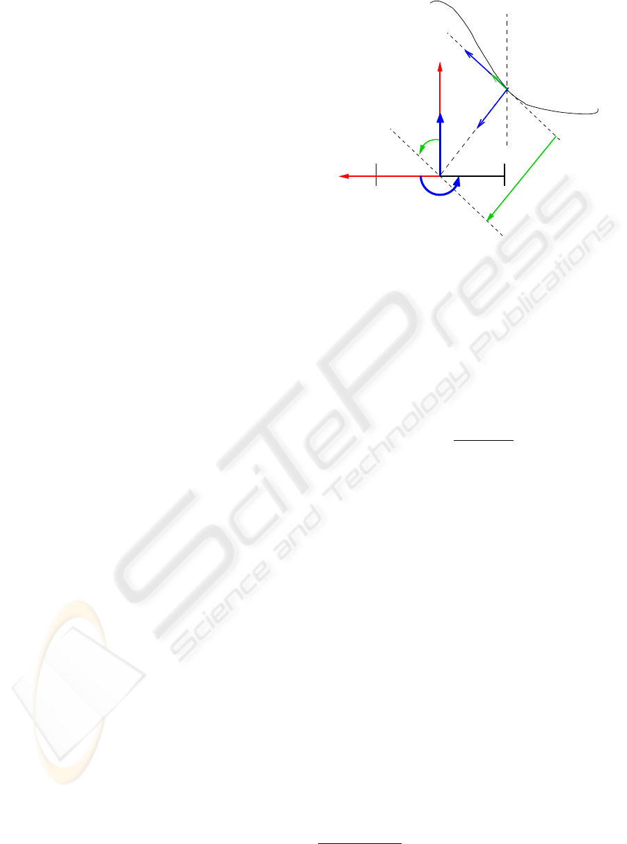
The robot is supposed to roll without slipping.

Whereas the avoidance strategy is based on a path fol-

lowing formalism, the robot kinematic model is ex-

pressed in a Frenet frame F

. Let M be the orthogo-

nal projection of O

on a curve ζ. We assume that the

distance from O

to ζ always remains smaller than

Figure 1: Robot kinematic model in a Frenet frame.

the minimal value of the curvature radius along ζ. In

this way, M is unique. F

is represented on Figure 1,

where s is the curvilinear abscissa associated to M on

ζ. e

and e

are respectively the lateral and the angu-

lar deviations of the robot with respect to ζ. Let c(s)

be the curvature of ζ at M . The robot motions are

described with respect to F

by the following kine-

matics equations:











˙s =

cos e

1 − e

c(s)

˙e

= u

sin e

˙e

= u

− ˙sc(s)

(1)

2.2 Observation Zone

Let us deﬁne a virtual zone, called observation zone

and surrounding the robot, as a planar curve ζ

lying

on Π , (O

, X

, Y

). The polar coordinates of

each point on Π will be denoted ρ for the module and

θ for the argument.

Let now f

be a continuous and derivable function:

[−π, π] 7→ IR

θ −→ ρ = f

(θ)

(2)

such that

∀θ ∈ [−π, π] , ρ > 0

clearly deﬁnes a virtual zone that surrounds O

Π. This virtual zone is a closed curve ζ

which marks

off a set Z with O

∈ Z

= inf {ρ > 0 | ρ = f

(θ)} (3)

given a set A, infA =

max {t ∈ [0 , +∞] | ∀a ∈ A , t < a}

A PATH PLANNING STRATEGY FOR OBSTACLE AVOIDANCE

439

obstacle

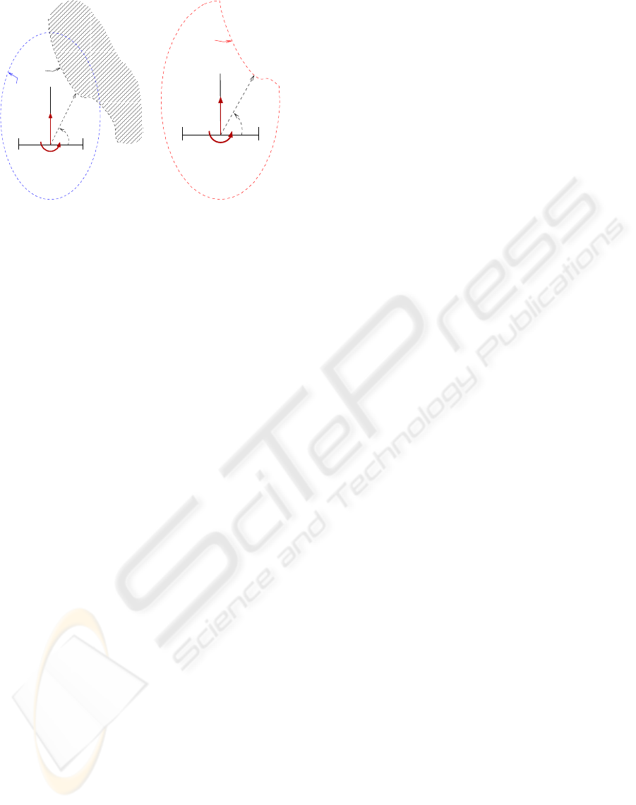
(a) (b)

Figure 2: Illustration of the deﬁnition of: (a) the observation

zone by ζ

, the obstacle shape by ζ

; (b) the free zone by

We assume now that an obstacle is known in F

a polar function f

in Π describing its shape. Let ζ

be the corresponding curve:

= inf {ρ > 0 | ρ = f

(θ)} (4)

deﬁnes the set O which contains the points lying on

the considered obstacle. If we assume that the robot

did not collide with the obstacle then O

6∈ O.

Figure 2(a) illustrates above deﬁnitions with an el-

liptic virtual zone and a single obstacle.

2.2.1 Uncontrolled Deformations

When an obstacle gets closer to the robot, it may

physically penetrate into the virtual zone. In this case,

Z ∩ O 6= ∅. We deﬁne the free set F as:

F = Z − O

Now consider the curve ζ

= min(ζ

, ζ

) (5)

is a closed curve, always deﬁned since ζ

is also

a closed curve and F is the inner set deﬁned by ζ

Note that ζ

can be considered as the result of the

deformation of ζ

by the uncontrolled intrusion of an

obstacle as illustrated by Figure 2(b).

2.2.2 Controlled Deformations

Till now, ζ

was only considered as a geometric curve

which did not depends on time since f

was ﬁxed.

However, it may be judicious to adapt the shape of

with the navigation context. Remembering that the

robot is guided by a navigation module, ζ

may be

deformed in a controlled mode by taking into account

the input control vector U

= [u

, u

] provided by

this module. Then the deﬁnition of f

(refer to equa-

tion (2)) has to be modiﬁed: ρ = f

(θ, U

For instance, an appropriated deformation should be

to control a scale factor on ζ

according to u

, in

order to extend the observation zone when the robot

goes fast. If the robot goes slowly, it probably navi-

gates in a cluttered or unknown space. In this case, it

has to be reactive to obstacles and its motions should

not be too much constrained so that it can carry on

making progress.

If we now consider the robot as a volumic object in-

stead of a single point, it appears necessary to con-

strain the controlled deformations of ζ

with a low

limit. This low limit can be seen as a security zone

that includes the robot.

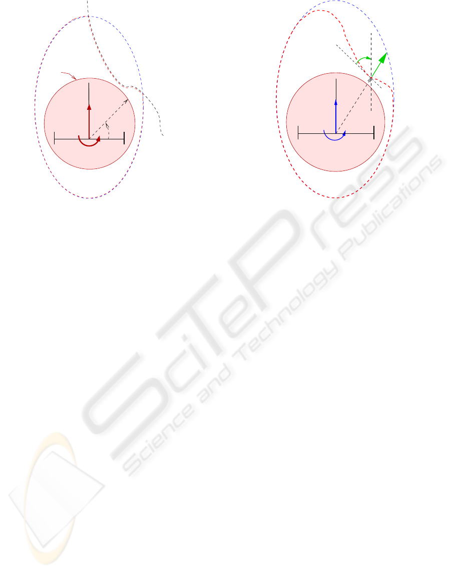
2.3 Security Zone

As the observation zone ζ

(refer to equation (3)), the

security zone is deﬁned as a closed curve ζ

. The

associated function f

is designed in order that ζ

closely ﬁts the area deﬁned by the orthogonal projec-

tion of the robot volume on Π.

is not deformable. From a practical point of view,

it must be designed according to the minimal range

that embedded sensor are able to provide accurately.

No obstacle has normally to come within ζ

, but if un-

fortunately it happens, the obstacle must be detected

to adapt the control strategy. This also implies that ζ

should be within ζ

as illustrated in the Figure 3. The

controlled deformations of ζ

are thus limited:

∀θ ∈ [−π, π] , f

(θ, U

) ≥ f

(θ) (6)

Seeing its functional interest, ζ

plays an important

rule for the control design.

3 CONTROL DESIGN

3.1 Control Strategy

The avoidance control law aims to drive the robot in

order to get F = Z.

Let M be a point of ζ

deﬁned as:

M , min {ζ

− ζ

} (7)

M is the orthogonal projection of O

on the piece

of curve ζ

which is not in ζ

. Note that if F = Z,

M = ∅. In this case, we consider that the coordinates

of M are not deﬁned; otherwise, we note (ρ

, θ

, 0)

the coordinates of M in F

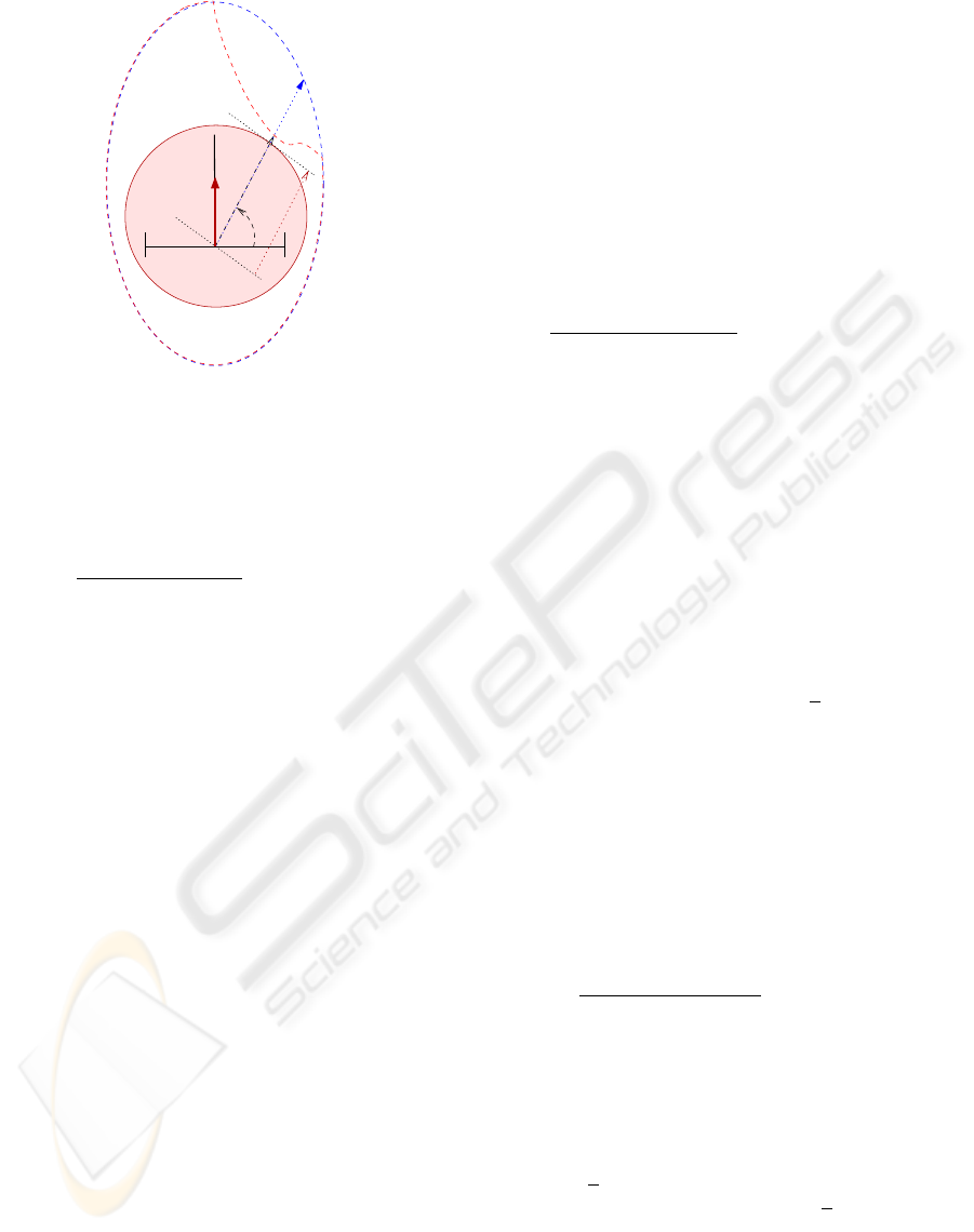
Now let us deﬁne the error e

which models the defor-

mation from ζ

to ζ

by the following signed distance

(see Figure 4):

= f

(θ

, U

) − ρ

(8)

ICINCO 2006 - ROBOTICS AND AUTOMATION

440

Figure 3: The security zone ζ

is a lateral deviation which may be regulated to

zero to push away the obstacles from the virtual zone.

Let us also deﬁne the angular deviation e

with re-

spect to the longitudinal axis X

as the orientation of

the tangent vector to ζ

at M . The avoidance con-

trol objective is to stabilize both e

and e

to zero.

This deﬁnes a path following problem. In the sequel,

this issue is addressed using the theoretic framework

of chained systems (Samson, 1995).

3.2 Lateral Control

The state space model (1) can be converted into a

chained system of dimension three:

, a

] = [s, e

, (1 − e

c(s)) tan e

] (9)

with a two dimensional control vector [m

, m

]

⊤

∈

. The derivative of such a chained system with

respect to time is:

(

˙a

= m

˙a

= a

˙a

= m

(10)

If this state vector is derivated with respect to a

, then

it appears that resulting kinematic system is linear. A

simple control which asymptotically stabilizes a

and

thus consists on a proportional state feedback:

= −m

− | m

| K

, (K

, K

) ∈ IR

+∗

(11)

, K

) determines the performances of the con-

troller and deﬁnes a settling distance for the regula-

tion of a

and a

to zero. These two gains control the

reactivity of the robot when avoiding an obstacle.

Figure 4: Lateral control: Deﬁnition of errors to be regu-

lated for obstacle avoidance.

In equation (11), m

appears as a parameter which

does not inﬂuence the regulation dynamic. m

is di-

rectly linked to u

by:

= ˙s = u

cos(e

) (12)

The system (10) leads to uncouple the controls m

and m

. This implies that u

and u

are also uncou-

pled. The rotational velocity resulting from the lat-

eral regulation of the robot with respect to the obsta-

cle will be denoted u

in the sequel. Independently

from u

, a longitudinal velocity u

can be used to

adapt the longitudinal velocity u

to the navigation

context.

3.3 Longitudinal Control

The value of the longitudinal velocity does not a

priori inﬂuence the lateral regulation performances.

Then, u

could take any value u

provided by the

navigation module without any dammage. From a

practical point of view, it is advantageous to reduce

it when the environment seems to become cluttered.

Firstly, this ensures that the robot can stop if an ob-

stacle is detected close to the frontier of the security

zone. Secondly, this allows to get more accurate and

stable data from sensors when obstacles come closer

to the robot. The strategy for longitudinal control

consists on applying an adaptative gain α on u

order to stop the robot if an obstacle is within de

security zone, and to get u

= u

if no obstacle is

observed within ̺

A PATH PLANNING STRATEGY FOR OBSTACLE AVOIDANCE

441

Figure 5: Longitudinal control.

α : [−π, π] 7→ [0, 1]

if M 6= ∅











α =

− f

(θ

)

(θ

) − f

(θ

)

if ρ

≥ f

(θ

)

α = 0 otherwise

otherwise

α = 1

(13)

and:

= α u

(14)

Of course, if the robot stops while a dynamic obsta-

cle intends deliberately to run into, the collision will

occur. At present, we do not focuses on this problem.

3.4 Global Control

As exposed in sections (3.2) and (3.3), the OAM pro-

vides a control vector U

= [u

, u

] which aims to

correct U

from a navigation module. u

is directly

linked to u

, however the computation of u

does

not take u

into account. The OAM must favor the

navigation module outputs if the local conﬁguration

of obstacles allows it. One can confere more impor-

tance to U

when an obstacle draws near the security

zone. Let U



, u



be the result of the cor-

rection of U

by the OAM. U

is computed according

to the following equations:







= u

= γu

+ (1 − γ)u

(15)

If γ is taken equal to α, near the frontier of the secu-

rity zone, the importance given to u

would be max-

imum while u

tends to zero. In order to get a more

reactive behavior, the deﬁnition of f

is modiﬁed as

∀θ ∈ [−π, π[ , f

(θ, U

) ≥ f

(θ) + ε (16)

where ε is a constant scalar which allows to keep a

zone around ζ

when u

is non-zero and the robot is

exclusively steered by u

γ : [−π, π] 7→ [0, 1]

if M 6= ∅











γ =

− f

(θ

) + ε

(θ

) − f

(θ

) + ε

if ρ

≥ f

(θ

) + ε

γ = 0 otherwise

otherwise

γ = 1

(17)

3.5 Singularities

The proposed control design conduces to some sin-

gularities which should not be ignored. They result

from the lateral control strategy. First, the point M

is not necessarily unique. Secondly, the curvature

c(s) is not deﬁned if f

is not two times derivable

at θ

. Last, e

may be equal to ±

. From a prac-

tical point of view, the ﬁrst two singularities can be

shunned. Indeed, curves ζ

and ζ

result from inter-

polation of scanning range sensors data. They are not

usually treated as analytic curves but as a set of sam-

pled points corrupted by measurement noises. Conse-

quently, M is not chosen among many points. How-

ever, if a choice has to be made, criteria can direct

it. The closest point to the X

axis, which directs

the longitudinal robot motion, can be privileged. Fur-

thermore, since curves are sampled with a constant

step ∆θ , the k

derivative f

of f

are computed as

(θ) =

k−1

(θ+h)−f

k−1

(θ−h)

, where h = n ∆θ and

n is a strictly positive integer. The curvature c(s) is

thus always deﬁned.

The third singularity corresponds to the case where

the robot goes orthogonally to an obstacle. The state

(9) is no more deﬁned and, as a consequence, not ei-

ther the control law (11). It is all the more problem-

atical that m

should exponentially increase since e

tends to ±

. To avoid such a conﬁguration, one can

impose m

= 0 when e

tends to ±

. In this way,

the longitudinal control law prevents the robot from

colliding with the obstacle.

ICINCO 2006 - ROBOTICS AND AUTOMATION

442

4 IMPLEMENTATION

This section illustrates the proposed approach from a

practical point of view. The framework proposed in

sections (2) and (3) was applied to assist the driving

of an indoor mobile robot equipped with a telemetric

sensors belt.

The OAM has been implemented on an external stan-

dard PC which wireless controls a Pioneer robot. This

robot is equipped with a eight sonars belt. Telemetric

data are acquired at f

= 10Hz. The control inputs

are also cadenced at f

. Telemetric data are collected

as eight range values, associated respectively to each

sensor. None ﬁltering is processed on these data and

none uncertainty on measures is taken into account.

4.1 Virtual Zones

The two virtual zones ̺

and ̺

are chosen as two

concentric circles. The diameter of the security zone

is set to φ

= 0.6m. In this way, ̺

surrounds every

sightless zone between two consecutive sensors. The

parameter ε is ﬁxed to 0.3m. The diameter φ

of ̺

linearly depends on u

. It is a priori limited by the

maximum range of sensors (i.e 3m). However, the

maximum value of φ

is set to φ

zmax

= 1m in order

to not constrain the robot motion when the obstacles

are far away from ̺

. Let u

cmax

be the maximum

longitudinal velocity of the robot then φ

is given by:

= (φ

+ 2ε)



1 −

max



+φ

max



max



4.2 Planning of a Straight Line

Although it is possible to interpolate the data at

each sample to obtain a smooth curve which roughly

delimits the set of obstacles observate by the sonars,

we refer the avoidance algorithm to a simple straight

line. This line determines ̺

. ̺

is deﬁned by the

point M and a vector ∆

. M is obtained from the

observations at time k : σ

= [σ

, σ

, . . . , σ

]

as the closest point to O

within the circle ̺

. ∆

depends on the navigation module outputs.

Let Ω

be the instantaneous steering

angle which should have directed the robot if it was

only guided by the navigation module. The vector

Ω

, where z

is the unitary vector which directs

the axis Z

, represents the directing vector of the

instantaneous robot motion. Let σ

be the range

data holden to estimate the point M. Another range

data is needed to determine a second point N to

build ̺

. The choice falls on σ

i+1

if θ

≥ Ω

i−1

otherwise. Then let θ

be the argument of

the vector

−−→

MN . If θ

> Ω

, then ∆

−−→

MN .

Otherwise, ∆

= Ω

. In this way, we take care

that the OAM does not servo the robot on a line from

which the navigation module would have a tendancy

to get the robot out of the way. If M is obtained from

or σ

, N may not exist. Then ∆

is forced to

be Ω

In the case of a straight line following, we have

∀s, c (s) = 0 which implies a simpliﬁcation of the

control design exposed in section (3.2). Equation (11)

leads to the following simple control law:

= −u

cos e

− | u

cos e

| K

tan e

This law ruled the robot motion during the experi-

ments which results are presented in the next section.

4.3 Results

We have validated the OAM with two kind of experi-

ments.

The ﬁrst one consists on a very simple robotic task. It

consists on going forward, with U

= [v, 0]

⊤

, where

v is a constant. We have tried for v a range of longitu-

dinal velocities from 0.1m.s

−1

to 0.5m.s

−1

, which is

a respectable value for an indoor robot. Initially, the

robot is placed in order to be directed to a wall, with

an incidence angle of approximately −

rad. The di-

ameter of the circular security zone is ﬁxed to 0.6m

while ε is set to 0.3m. In these conditions, the OAM

works as it is forecast in such a simple case.

The second task is more interesting. The robot is tele-

operated in ofﬁces and corridors of our laboratory and

the operator can not directly see the robot. He only

can see the image provided by an embedded frontal

camera which has an angle of view of 60deg. Im-

ages are wireless transfered, what implies some un-

expected and non constant delays on the visual feed-

back. In this case the OAM ensures the robot secu-

rity and assists the operator. However, circular virtual

zones rapidely appear unadequated. When an obsta-

cle comes closer to the robot from a side, the OAM

tends to correct the trajectory and unexpected oscil-

lations of the robot trajectory are induced. Elliptic

zones should be a solution to this issue.

5 CONCLUSION

This paper has presented the design and an implemen-

tation of an obstacle avoidance module (OAM) which

aims to act on the robot control inputs in order to pre-

serve the security of the robot when it is driven by

a navigation module which does not take explicitely

into account the possible presence of unexpected ob-

stacles.

The OAM is based on an original obstacle avoidance

A PATH PLANNING STRATEGY FOR OBSTACLE AVOIDANCE

443

approach. It consists on assigning to the robot a reac-

tive behavior by following a dynamically computed

path which results from the local observation of the

robot environment. None a priori model of obsta-

cles is needed since their shape can be estimated from

range data when the robot get closer to them. This es-

timated shape serves as reference of a path following

based control law which aims to pushing away obsta-

cles from a virtual zone. This zone is a closed curve

surrounding the robot and its shape can be modiﬁed

according to control inputs provided by the naviga-

tion module.

The approach has been illustrated in a simple case.

However, we have put it on the test in much more

complex contexts. Helped by the OAM, a user can

teleoperate the robot from a different room to the one

where the robot is navigating. The user can safely

drive the robot when he has only a limited view of the

cluttered navigation environment from an embedded

camera looking forward.

Although a simple case of implementation, based on

circular virtual zones, has been presented, many dif-

ferent shapes for virtual zones have been tested. No-

tably, ellipses appears as a very judicious choice. The

efﬁciency of the OAM should be improved by using

sensors as a laser range scanner since it can provide

more numerous and accurate range data. The pro-

posed formalism should then be implemented without

resorting to restrictive practical simpliﬁcations.

REFERENCES

Barraquand, J., Langlois, B., and Latombe, J. (1992). Nu-

merical potential ﬁeld techniques for robot path plan-

ning. IEEE Transactions on System, Man and Cyber-

netics, 22(2):224–241.

Blanc, G., Mezouar, Y., and Martinet, P. (2005). Indoor nav-

igation of a wheeled mobile robot along visual routes.

In IEEE International Conference on Robotics and

Automation, ICRA’05, Barcelona, Spain.

Braitenberg, V. (1984). Vehicles: Experiments in Synthetic

Psychology. The MIT Press, Cambridge, Massa-

chusetts.

Filliat, D., Kodjabachian, J., and Meyer, J.-A. (1999). Evo-

lution of neural controllers for locomotion and obsta-

cle avoidance in a 6-legged robot. Connection Sci-

ence, 11:223–240.

Khatib, O. (1986). Real time obstacle avoidance for ma-

nipulators and mobile robots. Int. Journal of Robotics

Research, 5(1):90–98.

Laumond, J. (1998). Robot motion planning and control,

volume 229, chapter Guidelines in nonholonomic mo-

tion planning, pages 1–54. Springer.

Samson, C. (1995). Control of chained systems. applica-

tion to path following and time-varying stabilization

of mobile robots. IEEE Transactions on Automatic

Control, 40(1):64–77.

Samson, C., Espiau, B., and Borgne, M. L. (1991). Robot

Control : The Task Function Approach. Oxford Uni-

versity Press.

Zapata, R., Lepinay, P., and Thompson, P. (1994). Reactive

behaviors of fast mobile robots. Journal of Robotic

Systems, pages 13–20.

ICINCO 2006 - ROBOTICS AND AUTOMATION

444