ON THE USE OF OPTIMIZATION METHODS FOR THE
MINIMIZATION OF FERTILIZER APPLICATION ERROR WITH
CENTRIFUGAL SPREADERS
Teddy Virin
§
, Jonas Koko
§§
, Emmanuel Piron
§
and Philippe Martinet
§§§
§
Cemagref
03150 Montoldre, France
§§
LIMOS, Universit
´
e de Blaise Pascal
63177 Aubi
`
ere cedex, France
§§§
LASMEA, Universit
´
e de Blaise Pascal
63177 Aubi
`
ere cedex, France
Keywords:
Optimization, Augmented lagrangian, Centrifugal spreading, Fertilizer application error.
Abstract:
Fertilizer application is one of the most important operations in agricultural production. Thanks to their low
cost and robustness, centrifugal spreaders are widely used to carry out this task. However, when distances be-
tween successive paths followed by the tractor in the field are not constant, application errors occur. These ones
generally cause waters pollution and economic issues. In this paper, to limit harmful environmental effects
and disastrous drop in production due to centrifugal spreading, we propose an approach based on optimiza-
tion techniques to improve the fertilization quality. An optimization criterion relying on a spatial distribution
model, obtained in previous works, is considered. To compute optimal parameters which should be used as
reference variables for the control of the spreader in the future, mechanical constraints are introduced. Faced
with a large scale problem, we use an augmented lagrangian algorithm combined with a l-bfgs technique.
Simulations results show low application error values comparing to fertilization inaccuracies found without
optimization.
1 INTRODUCTION
Fertilization operation is commonly achieved to apply
nutrients to make up the soil deficiencies and there-
fore enable a correct growth of plants in farmlands.
Centrifugal spreading is the main technique used to
distribute mineral fertilizers with respect to desired
doses calculated from agronomical and pedological
reasonings. This method permits to have uniform dis-
tributions as long as the trajectories followed by the
tractor equipped with spreader are parallel and regu-
larly spaced. Unfortunately, the use of this kind of
applicator is quickly limited when geometrical sin-
gularities, such as irregularly spaced tramlines, non
parallel paths or start and end of spreading, occur. In-
deed, at these spots, local application errors can be
observed. In some cases, over-application can lead
to an eutrophication phenomenon causing the disap-
pearance of aquatic species (Isherwood, 1998). More-
over, when the distributed amounts are below the pre-
scribed dose, the final production is often very low.
Thus, these statements lead the different governments
in Northern Europe to impose some strict rules as
specified in (Bruxelles, 2005). Confronted with these
requirements, many researches are carried out in or-
der to not only reduce dramatic environmental effects
but also increase margins in agricultural crop produc-
tion. In this study, we focus on a new approach based
on optimization techniques. We consider a cost func-
tion formalized from the actual spatial distribution
model instead of using the traditional method relying
on the best arrangement of transverse distribution. To
take into account the mechanical limits of applicator,
constraints are also considered. Thus, the computed
optimal parameters should be used as reference values
for future works dealing with the control of spreader.
This paper is organized as follows. The next section
exposes the centrifugal spreading principles and the
related drawbacks. In section 3, the cost function
modeling is dealt with. To solve the problem in an
efficient way, the problem decomposition and the op-
timization techniques are detailed in section 4. In the
124
Virin T., Koko J., Piron E. and Martinet P. (2006).
ON THE USE OF OPTIMIZATION METHODS FOR THE MINIMIZATION OF FERTILIZER APPLICATION ERROR WITH CENTRIFUGAL SPREADERS.
In Proceedings of the Third International Conference on Informatics in Control, Automation and Robotics, pages 124-129
DOI: 10.5220/0001212501240129
Copyright
c
 SciTePress

last section, because of more complicated phenomena
occurring in boundary zones, we apply this method
along parallel and non parallel trajectories only in the
main field body and expose simulation results.
2 CENTRIFUGAL SPREADING
DRAWBACKS
According to the soil and crops characteristics, agri-
cultural engineers state the amounts to be applied
within the farmland. These desired doses often takes
the form of prescribed dose map. This map depicts the
field which is virtually gridded and where each mesh
corresponds to the previously specified doses. Fertil-
ization aims to distribute nutrients so that the actual
spread doses get close to the prescribed ones. This
spreading regularity is above all performed by cen-
trifugal spreaders with double spinning discs which
eject fertilizers along each tramline in the field. The
functioning principles of these applicators are very
simple. Indeed, while the tractor progresses, fertiliz-
ers granulars contained in the hopper pour onto each
disc and are ejected by centrifugal effect.
Nowadays, with precision farming technologies, in
order to apply inputs according to the machine lo-
cation and a prescribed dose map, tractor-implement
combination is equipped with a GPS antenna, a radar
speed sensor and an actuator. The two first tools en-
able to know the tractor position and speed. Con-
cerning the actuator, it permits to control the fertilizer
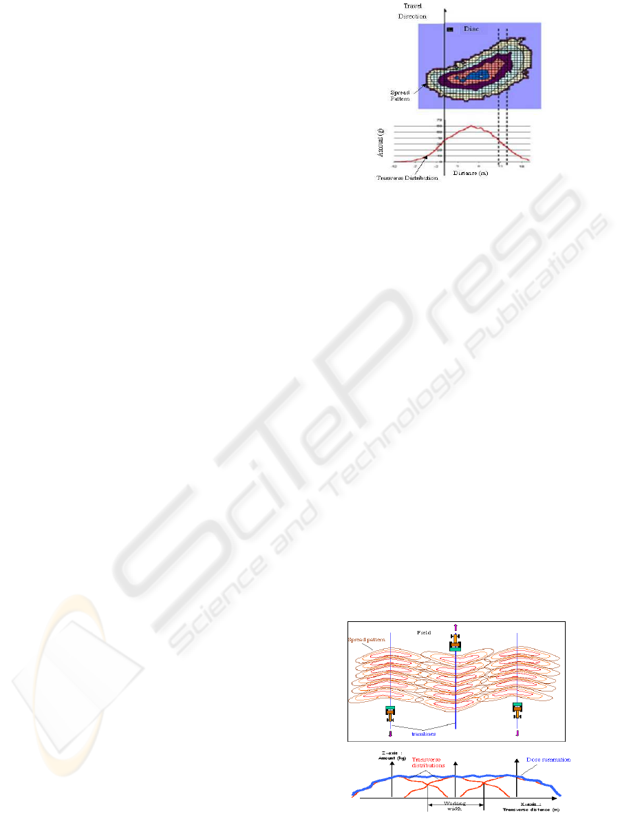
mass flow rate. The actual amount of applied fertiliz-
ers currently called spread pattern has an irregular dis-
tribution which is often underlined by the transverse
distribution curve obtained by summing the amounts
along each travel direction. An example of spread pat-
tern and its related transverse distribution for only one
disc are depicted in Figure 1. Thus, this spatial het-
eregeousness lead the tractor driver to follow outward
and return paths in order to have an uniform deposit
from transverse distribution summation for each suc-
cessive tramlines within the arable land. This strategy
is detailed in Figure 2. As we can notice, fertiliza-
tion strategy is essentially based on the best overlap-
pings of transverse distribution according to the dif-
ferent tractor trajectories. This method is applied for
experiments undertaken to evaluate fertilizer applica-
tion accuracy or to investigate device settings accord-
ing to tests procedures such as (ISO, 1985). So, these
procedures enable to select optimal machine settings
in order to obtain a regular deposit. Some studies re-
lying on these tests are also led to assess performance
of applicators like in (Yule et al., 2005). Deposits are
considered to be uniform when the distance between
two overlapping lines are equal to the distance sep-
arating two successive tramlines. Moreover, if this
Figure 1: Spread pattern (spatial distribution) and trans-
verse distribution (red curve).
condition is checked, overlapping lines are symmetry
axes which make two consecutive paths coincide. In
this case, the distance between two successive trajec-
tories, called working width, is said optimal. Unfortu-
nately, when applying this strategy in the field, the ac-
tual phenomenon occurring during spreading process
is ignored. Indeed, the deposit on the ground results
in fact from the accumulation of several amounts dis-
tributed for different spreader GPS positions. There-
fore, when geometrical singularities occur, like non
parallel paths or start and end of spreading, fertiliza-
tion application errors appear as illustrated in Figure
3(c) where results are obtained by simulating spread
patterns overlappings with settings imposed by manu-
facturers rules. To limit these issues, a solution could
be to look for optimal paths for the machine as in (Dil-
lon et al., 2003).
However, this kind of solution cannot be applied
when tramlines are already fixed by other agricultural
operations like sowing. So, it is clear that some ef-
forts must be done to achieve better spread patterns
arrangement according to geometrical constraints met
Figure 2: Fertilization strategy based upon transverse dis-
tribution summation.
ON THE USE OF OPTIMIZATION METHODS FOR THE MINIMIZATION OF FERTILIZER APPLICATION ERROR
WITH CENTRIFUGAL SPREADERS
125

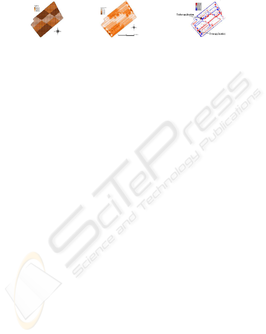
(a) Prescribed
dose map ob-
tained from
agronomical
considerations.
(b) Actual dose
map obtained by
applying the fer-
tilization method
based on adjust-
ment of transverse
distribution.
(c) Application errors
map calculated from the
difference between the
prescribed dose map and
actual dose map.
Figure 3: Application errors resulting from the reasoning based on the best transverse distribution investigation and not on
spread patterns overlappings.
in farmland during fertilization practice. The com-
puted adjustments should be continuously achieved
for each position of applicator by modifying its set-
tings. In this work, we study then a method which
permits to calculate optimal parameters to have the
best spread patterns arrangement within the field in
the presence of imposed tramlines.
3 COST FUNCTION
In order to develop a suitable optimization criterion,
we must consider the spread pattern model. This
model needs then the definition of some parameters
such as the time (t ∈ R), the spatial domain, in other
words the field, (Ω ∈ R
2
), the path (s(t) ∈ Ω), the
coordinates of points (x ∈ Ω), the distance between
s(t) and x (r(x, t) ∈ R) and the angle between
−−−→
s(t)x
and s(t) (θ(x, t) ∈ R). The spread pattern shown in
Figure 1, is currently defined by its medium radius
and medium angle. The first parameter, varying with
the speed of disc, corresponds to the distance between
the disc centre and the spread pattern one while the
second, modifiable with the fertilizers dropping
point on the disc, states the angle between the travel
direction and the straight line passing through the
disc centre and the spatial distribution one. Here, the
respective mass flow rates for the right and left discs
are defined by m(t) and d(t). ρ(t) and ξ(t) stand
for the medium radius related to the right and left
discs respectively. At last, ξ(t) and ψ(t) correspond
to the right and left discs medium angles. All these
parameters are defined in R. By assuming σ
r
and σ
θ
to be the respective constant standard deviations for
the medium radius and the medium angle, we can
calculate the right and left spatial distributions q
r
and
q
l
, according to (Olieslagers, 1997), as:
q
r
(x, m(t), ρ(t), ϕ(t)) = τ · exp(−A(x, t)
2
/a)
· exp(−B(x, t)
2
/b) (1)
q
l
(x, d(t), ξ(t), ψ(t)) = κ · exp(−C(x, t)
2
/a)
· exp(−D(x, t)
2
/b) (2)
with A(x, t) = r(x, t) − ρ(t) (3)
B(x, t) = θ(x, t) − ϕ(t) (4)
C(x, t) = r(x, t) − ξ(t) (5)
D(x, t) = θ(x, t) − ψ(t) (6)
and where a = 2σ
2
r
, b = 2σ
2
θ
, τ = m(t)/(2πσ
r
σ
θ
)
and κ=d(t)/(2πσ
r
σ
θ
). To simplify notations,
we define M (t) = (m(t), d(t)) ∈R
2
, R(t) =
(ρ(t), ξ(t)) ∈R
2
and Φ(t) = (ϕ(t), ψ(t)) ∈ R
2
. The
global distribution is then obtained as the summation
of right and left contributions:
q
tot
(x, M (t), R(t), Φ(t)) = q
r
(x, m(t), ρ(t), ϕ(t))
+q
l
(x, d(t), ξ(t), ψ(t)) (7)
Thus, the actual distributed dose Q ∈ R
2
during the
interval of time (0, T ) for single tramline can be cal-
culated as:
Q(x, M, R, Φ)=
Z
T
0
q
tot
(x, M (t), R(t), Φ(t)) dt (8)
If Q
∗
stands for the prescribed dose, the cost function
to be minimized is given by:
F (M, R, Φ) =
Z
Ω
[Q(x, M, R, Φ) − Q
∗
]
2
dx (9)
Given that (9) cannot be calculated in an analytical
way, discretization is necessary. So, Ω is gridded
so that Q and Q
∗
can be computed with bilinear ap-
proximations. A temporal discretization is also car-
ried out. This is done by dividing the interval (0, T )
ICINCO 2006 - INTELLIGENT CONTROL SYSTEMS AND OPTIMIZATION
126

into n elements with equal length δ = T/n. We
can then define t
j
= jδ with j = 0, 1, ..., n. Con-
sequently, we can assume M
j
= M(t
j
), R
j
= R(t
j
)
and Φ
j
= Φ(t
j
). The corresponding vectors are de-
fined as M = [M
0
· · · M
n
]
T
, R = [R
0
· · · R
n
]
T
and
Φ = [Φ
0
· · · Φ
n
]
T
. In order not to untimely solicit ac-
tuators, constraints are introduced. So, the functions
M, R and Φ and their time derivative are subject to
bound constraints. The set of solutions is then defined
by S =

(M , R, Φ) ∈ R
6(n+1)

so that:

















M
min
≤ M ≤ M
max
R
min
≤ R ≤ R
max
Φ
min
≤ Φ ≤ Φ
max
|M
i+1
− M
i
| ≤ αδ
|R
i+1
− R
i
| ≤ βδ
|Φ
i+1
− Φ
i
| ≤ γδ,
(10)
where α, β and γ are known parameters fixed with
respect to the machine mechanical characteristics. We
obtain then a nonlinear programming problem given
by:
(P) min
(M ,R,Φ)∈S
F (M , R, Φ) (11)
The set S is in our case bounded closed. Thus, ac-
cording to the Weierstrass theorem, the problem (P)
has at least one solution. In most cases, there exist
several tramlines and the actual distributed dose for
all trajectories is then obtained by the summation of
the applied dose for each indexed k path:
Q(x, U )=
w
X
k=1
Q
k
(x, U ) (12)
withQ
k
(x, U )=
Z
t
k
f
t
k
i
q
tot
(x, M (t), R(t), Φ(t))dt(13)
and where U = (M, R, Φ). Here, w is the number
of paths and the trajectories s
k
(t) are assumed to be
defined in the interval (t
k
i
, t
k
f
). If we consider also
the definitions of M
k
j
= M(t
k
j
), R
k
j
= R(t
k
j
), and
Φ
k
j
= Φ(t
k
j
) we can then use the discretization tech-
niques as before. Consequently, from these defini-
tions, optimization in the whole field considering all
paths can be carried out by solving the problem (P).
4 METHODOLOGY OF
OPTIMIZATION
Fields mostly include many tramlines several hundred
metres long. If we apply the discretization scheme
previously detailed, we are confronted with a large
scale problem. Indeed, in our case, like most pre-
scribed dose map, the field is 1 m gridded. To lose
informations as little as possible, 2 samples of pa-
rameters per elementary mesh are computed. So if
we consider for example only 4 tramlines 100 m long
within the farmland, after discretization, the number
variables raises to 4800. From this statement, it is
clear that solving the optimization problem without
decomposition is prohibitive. Let us precise some no-
tations before the decomposition explanations:
K
1
= {k ∈ N| 1 ≤ k ≤ w} ,
K
2
= {k ∈ N| 1 ≤ k ≤ w − 1} ,
K
3
= {k ∈ N| 2 ≤ k ≤ w} ,
L
1
= {l ∈ N| ∀z ≥ 2 ∈ N, 1 ≤ l ≤ z} ,
L
2
= {l ∈ N| ∀z ≥ 2 ∈ N, 2 ≤ l ≤ z} ,
Ω =
S
k∈K
1
Ω
k
, Ω
k
=
S
l∈L
1
Ω
k
l
,
with Ω
k
∈R
2
the k
th
subdomain of Ω, and Ω
k
l
∈R
2
the
l
th
subdomain of Ω
k
. Here, we decompose the prob-
lem so that each path s
k
(t) is individually dealt with.
So, the subdomains Ω
k
are defined so that:
∂Ω
k
∩ Ω
k+1
= s
k+1
(t), ∀(k, t) ∈ K
2
× (t
k+1
i
, t
k+1
f
)
∂Ω
k
∩ Ω
k−1
= s
k−1
(t), ∀(k, t) ∈ K
3
× (t
k−1
i
, t
k−1
f
)
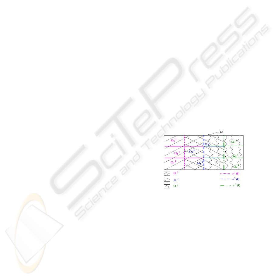
In order to make easier to understand the spatial de-
composition, Figure 4 illustrates the example of three
parallel tramlines in a domain Ω with a rectangular
geometry.
Figure 4: Rectangular domain Ω divided into 9 subdomains
Ω
k
l
, 1 ≤ l ≤ 3, 1 ≤ k ≤ 3.
Moreover, if we assume the vectors M
k
l
, R
k
l
, Φ
k
l
to be the respective restrictions of M , R and Φ in the
subdomain Ω
k
l
, we can also define also the set S
k
l
as
the restriction of S in the same subdomain. By tak-
ing into account the symmetries conditions exposed
in section 2, the natural decomposition of (P) is given
by:
(P
′
)

min
P
z
l=1
P
w
k=1
J
k
l
(x, M
k
l
, R
k
l
, Φ
k
l
)
(m
k
l
, R
k
l
, Φ
k
l
)∈S
k
l
, (l, k) ∈ L
1
×K
1
(14)
where
J
k
l
(x, M
k
l
, R
k
l
, Φ
k
l
) =
Z
Ω
k
l
[Q
k
l
(x) − Q
∗
]
2
dx (15)
ON THE USE OF OPTIMIZATION METHODS FOR THE MINIMIZATION OF FERTILIZER APPLICATION ERROR
WITH CENTRIFUGAL SPREADERS
127

with Q
k
l
(x) the actual distributed dose within Ω
k
l
tak-
ing into account not only the amounts already ap-
plied in Ω
k−1
l
and Ω
k
l−1
but also the future distributed
dose along the path s
k+1
(t) which is predicted so that
it respects the symmetries properties previously ex-
plained. The problem (P
′
) is an optimization prob-
lem subject to inequality constraints. For (l, k) ∈
L
1
× K
1
, to minimize the functional J
k
l
we consider
then the problem (P
ineq
) defined as:
(P
ineq
)



min J
k
l
(M
k
l
, R
k
l
, Φ
k
l
)
u
j
≤ h
j
(M
k
l
, R
k
l
, Φ
k
l
) ≤ v
j
,
j = 1, 2, ...dim(M
k
l
)
(16)
where h
j
denotes the j
th
double inequality, u
j
and
v
j
its lower and upper bound. In order to obtain
an acceptable solution after algorithm execution and
avoid solving the problem which consists in determin-
ing saturated constraints, we choose to apply an aug-
mented lagrangian algorithm (Bertsekas, 1982) asso-
ciated with a l-bfgs technique shown to be efficient
with large scale optimization problem (Byrd et al.,
1994). Moreover, desirous of obtaining the best fer-
tilizer application in the field, it is important to note
that the optimization algorithm is not time-bounded.
5 APPLICATION
Here, we focus essentially on main fiel body applica-
tion and not on boundaries area where more complex
phenomena occur. A constant prescribed dose fixed
at 100 Kg/Ha is considered because even in the case
of uniform desired rate, application errors appear. The
speed of tractor is also constant and equal to 10 Km/h.
The studied farmland is illustrated in Figure 5.
0 50 100 150 200
−100
−50
0
50
100
x−coordinate (m)
y−coordinate (m)
main field body trajectories
headlands
boundaries
N
1
2
3
4
5
6
P
Path number P
Figure 5: Field with parallel and non parallel tramlines.
The default working width is fixed at 24 m. A nar-
rowing occurs at the end of the first path. The distance
between the 4
th
and 5
th
tramlines is 23 m while it is
equal to 21 m between the 5
th
and 6
th
trajectories. In
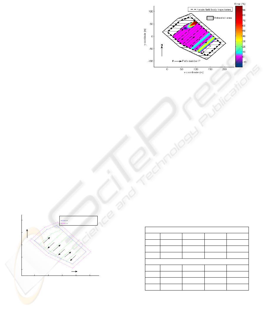
practice, the manufacturers settings do not vary dur-
ing time and are determined to be optimal with 24 m
working width. With these settings, we obtain errors
shown in Figure 6. As we can notice, over-application
areas appear on the left and the right of the 4
th
tram-
Figure 6: Application errors obtained with the manufactur-
ers settings.
line. Over-dosage is very important at the end of the
first path and almost reaches 95%. Futhermore, we
can distinguish an under-application zone slightly be-
low the break-point which marks the travel direction
change for this same trajectory. Everywhere else, er-
ror is included between -6% and +7% and is then ac-
ceptable. To reduce these fertilization errors, we ap-
ply our optimization methodology as detailed in the
previous section making sure that the considered me-
chanical constraints gather the characteristics of the
most used spreader. As in practice, for consecutive
parallel tramlines, optimal parameters are computed
so that they are time independent. So, calculated vari-
ables for the paths 3 to 6 are constant during time and
are recapitulated in Table 1. These values are very
close to actual current values.
Table 1: Optimal values for successive parallel tramlines
(M
f
: Mass Flow Rate (Kg/min); R
m
: Medium Radius; θ
m
:
Medium Angle (
◦
)).
Left Disc
Path 3 Path 4 Path 5 Path 6
M
f
19.32 17.92 19.41 20.6
R
m
15.13 14.61 14.7 15.17
θ
m
-20.78 -20.96 -19.66 -19.79
Right Disc
Path 3 Path 4 Path 5 Path 6
M
f
20.7 21.24 17.26 16.95
R
m
15.49 15.55 14 14
θ
m
18.93 18.37 18.61 18.79
Unlike the previous paths, optimal variables for the
two first trajectories are dependent time. The opti-
mized parameters for the first path are shown in Fig-
ure 7. The parameters for the left and right discs
appear respectively on the left and the right. As ex-
pected, after the travel direction change, the medium
radius drops. For the left disc, the mass flow rate
ICINCO 2006 - INTELLIGENT CONTROL SYSTEMS AND OPTIMIZATION
128

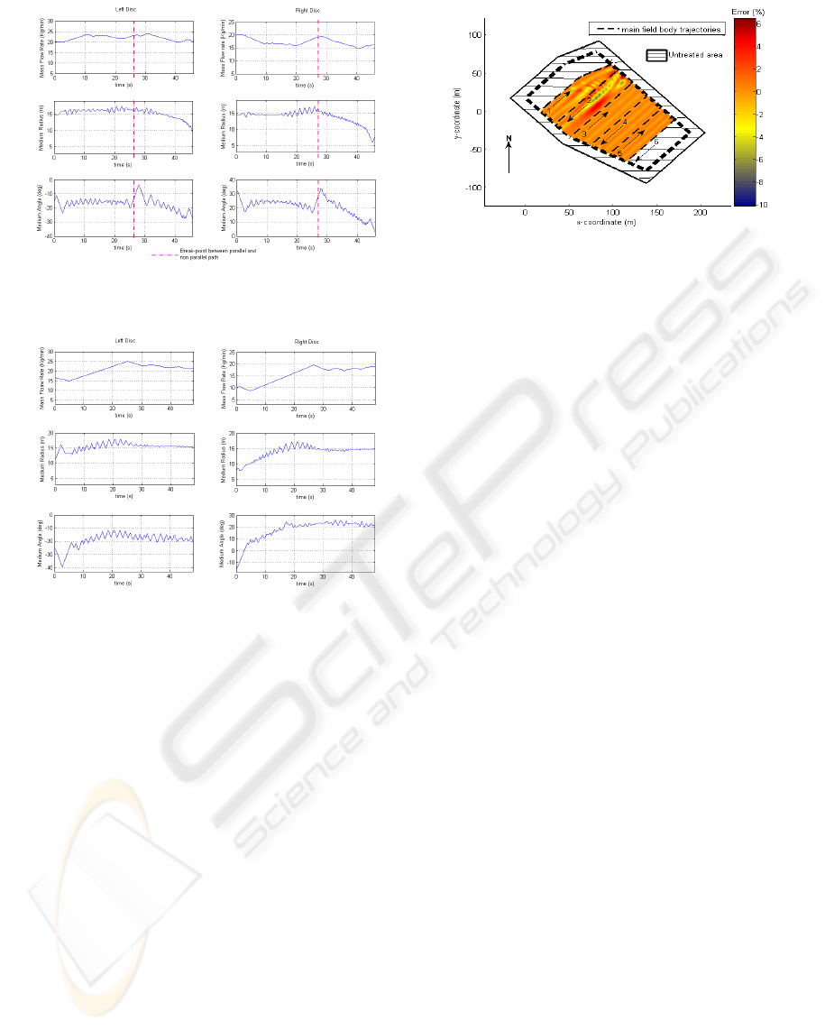
Figure 7: Optimal parameters for the first path.
Figure 8: Optimal parameters for the second path.
slightly varies around break-point and seems not to
be affected by the occurring narrowing. However,
for the right disc, it increases before the break-point
and drops after this one. Concerning the medium an-
gle, a similar evolution is observed around this point.
Figure 8 shows an increasing of all parameters for
each disc. This phenomenon can be explained by the
narrow pass occurring when the tractor comes in the
main field body. The values reached after stabilization
are close to the ones set by manufacturers with 24 m
spaced parallel trajectories.Figure 9 exposes a simu-
lation result in the main field body with the optimized
parameters. As we can notice, application errors are
reduced comparing to the ones exposed in Figure 6.
Optimization leads to errors included between -10%
and +6.3%, which is very satisfying with regard to
environmental and economic requirements.
6 CONCLUSION
A new method for optimization of fertilizer applica-
tion by centrifugal spreaders has been presented. To
Figure 9: Application errors obtained after optimization.
make sure that optimized parameters respect the ac-
tual process and can be used as reference variable for
the future control of the machine, bounds constraints
have been considered. Given the large scale prob-
lem resulting from the discretization, we have decom-
posed it and applied an augmented lagrangian algo-
rithm with a l-bfgs technique. Optimal parameters en-
able to really limit application errors. Future studies
are needed to optimize spreading process in bound-
aries zones. The computed variables for the whole
field should then significantly enhance spreading ac-
curacy.
REFERENCES
Bertsekas, D. P. (1982). Constrained Optimization and La-
grange Multipliers Methods. Academic Press, New
York.
Bruxelles (2005). Mise en oeuvre de la directive 91/676/cee
- pollution par les nitrates a partir de sources agricoles.
Byrd, R. H., Nocedal, J., and Schnabel, R. B. (1994). Rep-
resentations of quasi-newton matrices and their use
in limited memory methods. Mathematical Program-
ming, 63:129–156.
Dillon, C. R., Shearer, S., Fulton, J., and Kanakasabai, M.
(2003). Optimal path nutrient application using vari-
able rate technology. In Proc. of the Four th European
Conference on Precision Agriculture, pages 171–176.
Isherwood, K. F. (1998). Mineral Fertilizer Use and the
Environment. IFA.
ISO (1985). ISO 5690/1 Equipment for distributing fertil-
izers - Test methods - Part 1: Full width fertilizer dis-
tributors. International Organization for Standardiza-
tion, Geneve.
Olieslagers, R. (1997). Fertilizer distribution modelling for
centrifugal spreader design. PhD thesis, K.U. Leuven.
Yule, I., Lawrence, H., and Murray, R. (2005). Performance
of fertiliser spreading equipment for precision agricul-
ture applications. In 1st International Symposium on
Centrifugal Fertiliser Spreading, pages 10–18.
ON THE USE OF OPTIMIZATION METHODS FOR THE MINIMIZATION OF FERTILIZER APPLICATION ERROR
WITH CENTRIFUGAL SPREADERS
129