
CONSIDERATIONS FOR SELECTING FUNCTIONS AND
TERMINALS IN GENETIC PROGRAMMING FOR
FAULT-DETECTION IN EMBEDDED SYSTEMS
Matej
ˇ
Sprogar, Domen Verber, Matja
ˇ
z Colnari
ˇ
c
FERI, University of Maribor
Smetanova ul. 17, 2000 Maribor, Slovenia
Keywords:
Genetic programming, embedded systems, fault detection, monitoring cell.
Abstract:
The article describes the terminals and functions used by genetic programming to discover specific parameters
for fault-detection in embedded control systems design. Choice of different functions and terminals affects
the convergence speed. The state of embedded controller is mapped into a space of valid/invalid points and
genetic programming is used to divide the space into hypercubes that can be used to trivially recognize faults
during system operation. The fault-detection logic operates by monitoring the input and output variables
of the embedded controller. It is based on acquired and built-in knowledge about the normal behaviour in
order to detect abnormalities. The fault-detection problem is approched by the use of monitoring cells, which
implement the system supervising logic.
1 INTRODUCTION
Embedded control systems are present in all mod-
ern technological products with a strong position
even in safety critical environments. Highly depend-
able programmable electronic systems for safety crit-
ical embedded control and regulation applications are
mandatory. Due to the complexity of the control sys-
tems faults are an unavoidable fact. A discipline that
handles faults is called “fault management”. One
possibility to implement the fault-detection (a fault-
management technique) is to use a “monitoring cell”
(MC), which monitors the validity of inputs and out-
puts and (possibly) the internal states of the control
process. As a result, the fault-status is reported to a
higher fault management layer.
Run-time faults must be recognized by the fault-
detection mechanism of the MC. Such faults are the
most difficult to discover because they are a con-
sequence of totally unpredictable events or chain of
events. One way to detect run-time faults is to observe
whether the system behaves normally at all times.
The system is observed during normal operation by
recording all inputs, outputs and internal states which
are believed to affect its future behavior. Then a ma-
chine learning technique can be used to “learn” the
normal behaviour from collected data. Genetic algo-
rithms (GA) are the most easily applied evolutionary
paradigm to solve this problem, yet the article sets
focus on genetic programming (GP) because GP’s
evolved programs closely resemble the fault-detecting
functions of MCs and are therefore of special interest.
Section 2 describes the concepts behind the moni-
toring cell. Next the importance of selecting appropri-
ate functions and terminals for GP is emphasized. In
section 3 evolutionary computing (EC) is used to dis-
cover fault-detecting functions for monitoring cells.
For GP various functions and terminals are discussed.
2 EVALUATION OF THE
MONITORED SIGNALS
The monitoring cell effectively performs some eval-
uation function. A proper evaluation function can be
constructed in different ways. As a basic evaluation,
the integrity of each individual signal is verified. The
information on its basic properties is acquired from
the system specifications, technical documentation or
similar sources. This way at least information on the
data ranges – valid and invalid values of different sig-
nals – is extracted.
A more thorough validation of the system should
be performed to make sure that outputs are consistent
with the inputs. For this, the properties of transforma-
142
Šprogar M., Verber D. and Colnari
ˇ
c M. (2006).
CONSIDERATIONS FOR SELECTING FUNCTIONS AND TERMINALS IN GENETIC PROGRAMMING FOR FAULT-DETECTION IN EMBEDDED
SYSTEMS.
In Proceedings of the Third International Conference on Informatics in Control, Automation and Robotics, pages 142-147
DOI: 10.5220/0001215101420147
Copyright
c
SciTePress

tion function of the system must be known. To learn
the behaviour of the control function two general ap-
proaches are possible: to derive it analytically from
the available explicit knowledge about the process, or
to learn it by observation. In the latter case, the moni-
tored control system is observed during an interval of
valid operation to produce a learning set L consisting
of n instances s, each instance representing separate
input signals to the MC. This instance is actually a
point in a D-dimensional space, where D is the count
of signals in instance s.
The learning dataset L is a set of instances of
(co-related) signals and MC’s task is to determine
whether a previously unseen instance s belongs to the
space of known valid instances or not (a classifica-
tion/clustering problem). The MC’s limited process-
ing abilities mostly do not support the use of complex
rules for that purpose. The monitoring function can
be created off-line and a sequence of simple compar-
isons, which is sufficient to determine if a point lies
within a faulty region or not, can then be executed by
the MC during system operation.
Assuming the learning set includes all relevant sig-
nals then the simplest general clustering solution is
a hypercube – a generalization of the cube within D
dimensions. The smallest hypercube that includes
all learning instances from L is actually the space S
of all possible states of the control system. Beside
L’s (valid) learning instances, S contains plenty of
other points, most of which are descriptions of faulty
states of the control system. Learning algorithm has
to group (cluster) the valid points into smaller hyper-
cubes with mostly valid points. The learning process
can result either in (1) one, (2) too-many, or (3) few
hypercubes. If (1) then no optimization was per-
formed and all instances are always proclaimed valid.
This is possible if L ∼ S. If (2) the hypercubes are
too small and fail to group related instances. This is
a non-general partitioning of space S over-fitting the
learning set. Such hypercubes fail to classify correctly
most of the valid points not included in L. This is
mainly because no relations between instances exist
or the collected dataset does not include all relevant
signals for fault-detection. Few hypercubes (3) parti-
tion the space S into valid/invalid regions.
In general this is a multi-objective optimization
problem with conflicting goals – many small hyper-
cubes have low classification error yet they fail to
generalize and require more (scarce) computing re-
sources. Depending on hardware MC implementa-
tion, the MC can perform only a limited number
of point-in-hypercube tests. Therefore certain hy-
percubes will include noise (instances of the invalid
type).
2.1 Establishing the Monitoring
Function
From the learning set L the monitoring evaluation
function E must be constructed using a combination
of optimization, unsupervised learning and classifica-
tion techniques. Final solution must be verifiable in
order to be allowed for use in an embedded control
system.
All machine learning techniques are able to ex-
tract information from the learning data. Most of
them (e.g. K-means or minimal spanning tree clus-
tering algorithms, support vector algorithms, neural
networks), however, tend to produce overly complex
solutions unsuitable for MC implementation. The hy-
percubes paradigm suits the MC well and discovery of
hypercubes can be trusted to any evolutionary compu-
tation technique. Although several evolutionary tech-
niques (e.g. genetic algorithms or evolution strategies
(Banzhaf et al., 1998)) can be used, the focus here is
on GP as it is the only evolutionary paradigm capable
of evolving a complete fault-detection logic.
3 USING EC TO DISCOVER
FAULT-DETECTION RULES
The basic difference between GA and GP is that GAs
directly produce solutions according to some pre-
defined structure, while GP produces a self-structured
computer program that effectively calculates a desired
output for particular inputs. GP’s program is therefore
similar in concept to the MC’s monitoring function.
In order to use EC to discover the monitoring cell’s
evaluation function, a description of controller’s be-
haviour is needed. Normal operation of the controller
is described by the empirical learning set L. Genetic
programming could be used as a symbolic regression
tool to discover the symbolic expression that satisfies
the data points in the learning set. However, the hid-
den symbolic expression is probably a complex struc-
ture consisting of numerous mathematical operations
and functions (e.g. trigonometric functions) and is
probably too complex to be implemented in MC.
For monitoring cells the partitioning of the space
of all possible signals into two disjoint spaces S
−
and S
+
is required – space S
+
includes all points
(instances) from the learning set and thus describes
the “normal” states of the controller; S
−
includes no
such points and therefore represents a space of possi-
ble faults (even if system produces signals belonging
to S
−
, the system itself is not necessarily experienc-
ing a fault).
The example used throughout this section is based
on some unknown calculation C using a single scalar
CONSIDERATIONS FOR SELECTING FUNCTIONS AND TERMINALS IN GENETIC PROGRAMMING FOR
FAULT-DETECTION IN EMBEDDED SYSTEMS
143
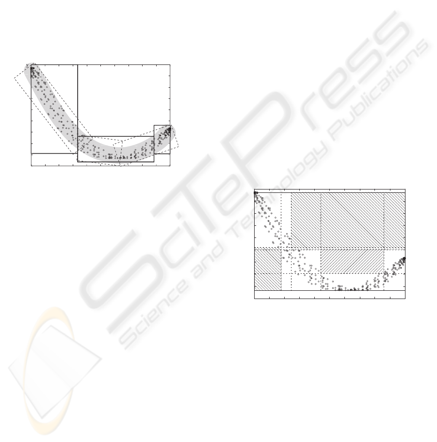
input x to produce a scalar output y = C(x). The
behavior of the example system using function C was
recorded to obtain a learning set L with 316 (x, y)
points displayed in Fig. 1. The coordinates in L
are limited: −10 ≤ x ≤ 10 and −32 < y < 775.
The relationship between x and y coordinates is un-
known, yet human can easily draw a clustering region
(marked with grey). This same region can be mostly
covered by three inclined dashed hypercubes S
′
0
, S
′
1
and S
′
2
. The approximation using three upright hyper-
cubes S
0
, S
1
and S
2
covers not only L but also many
unspecified points in S. The remaining space S
−
is
free of any recorded valid points. A general MC has
only enough processing power to test whether a point
belongs to an upright hypercube.
-100
0
100
200
300
400
500
600
700
-10 -8 -6 -4
-2
0
2
4
6
8
x
700
S
0
S
1
S
2
S'
2
2
S'
S'
1
1
S'
0
0
S
-
Figure 1: Dependency of y on x in learning set L. Cluster-
ing done by a human is marked with grey.
By using n upright hypercubes S
i
the monitoring
cell can perform only a very rough detection of faults.
The S
0
, for example, covers a large area designated as
invalid by a human expert. The optimization task is to
group available valid points into one or more hyper-
cubes while keeping the error (count of invalid points
inside the hypercubes) at a low level. Problem is that
it is impossible to determine if a hypercube includes
any invalid points because there are no invalid points
in L to verify this assertion.
It is possible, however, to invert the problem and
look for a hypercube H
i
which contains no valid
points: H
i
∩ L = ∅. This inverted task results in a
hypercube H
i
⊆ S
−
, contrary to the original opti-
mization task of producing a hypercube S
i
⊆ S
+
.
The machine learning algorithm must therefore di-
vide the space S into two mutually exclusive hyper-
spaces S
−
and S
+
in a way which maximizes the
hyper-space S
−
that consists of a finite number of hy-
percubes H
n
. For the GP to evolve a computer pro-
gram, which calculates the n hypercubes H
i
needed
by the MC, a function set and terminal set are needed
which produce 2nD coordinates (each hypercube is
uniquely defined by two opposite corners, each cor-
ner point with D scalar coordinates, respectively).
A similar approach to hypercubes is a matrix ap-
proach – each dimension (d
i
, i = 1..D) is divided into
I
i
intervals and the (hypercube) cells M
k
inside the
matrix represent clustering regions. A cell that con-
tains at least one valid sample represents a valid hy-
percube. This approach is simpler than the hypercube
approach, but can have more generalization difficul-
ties.
3.1 Optimization Using Genetic
Algorithm
GA is the simplest evolutionary optimization ap-
proach for hypercube sizing and positioning. Sup-
pose the MC hardware is able to execute enough in-
structions to test the inclusion of a point in three hy-
percubes, each hypercube being defined by two op-
posite corner points. For three hypercubes 6 points
in the 2-D space S are needed and GA has to pro-
duce 6 (x, y) pairs within the specified range (S =
[−10, 10] × [−31, 775]). Genetic algorithm typi-
cally operates with fixed-size bit strings, which are
first transformed into x, y pairs and then into hy-
percubes. Fitness function simply returns the score
|H
1+2+3
|/(err+1), where the |H
1+2+3
| operator re-
turns the size of the hypercube H
1+2+3
, and err is the
number of valid samples therein.
-100
0
100
200
300
400
500
600
700
y
-10 -8 -6 -4 -2 0 2 4 6 8 x
H
2
H
3
H
1
Figure 2: H
1
, H
2
and H
3
produced by OpenBeagle GA
using fixed-length bit strings (12 bits/coordinate, P=50,
G=1000).
Fig. 2 shows the results obtained from GA using
the OpenBeagle library (Gagne and Parizeau, 2006).
This same picture also shows the matrix of 20 cells,
which are designated by a dashed lines, and their par-
titioning of the search space S according to intervals
as determined by three hypercubes.
3.2 GP: Basic Scalar Functions and
Terminals
To use GP several prerequisites must be met, includ-
ing the closure and sufficiency property of the func-
ICINCO 2006 - INTELLIGENT CONTROL SYSTEMS AND OPTIMIZATION
144
tions and terminals (Koza, 1992). The most straight-
forward and general GP approach is to use the basic
scalar function set and terminal set to produce hy-
percube coordinates (+, −, ∗, /). Basic terminal set
of T = 0, 1 can be extended with basic problem-
specific constants ( x
min
, x
max
. . .) and ephemeral
(Koza, 1992) constants. This approach suffers from
the following problems:
• Ignorance of the “smaller” search space S; by us-
ing the basic functions and terminals the search
takes place in the range of underlying scalar co-
ordinate data-type rather than inside the bounded
search space S.
• Produces only one value.
• Has low convergence speed.
Advantages of this approach are:
• Is most generally applicable and is not limited by
any assumptions about the problem.
• Is supported by most available GP libraries and
therefore easy to implement – this is the basic kit
in all GP implementations.
The first problem is the search through the definition
space of the data-type rather than through problem
space S. This is because GP is searching for a com-
puter program that calculates values in the space of
all numbers, not in the range of valid numbers as de-
fined by S. For example, to calculate any x coordi-
nate for the H
1
hypercube from Fig.1, the program is
not limited to the [−10, 10] range; GP actually gen-
erates expressions for the full data-range of the data
type (e.g. float). A solution is to use an artificial map-
ping of calculated values into valid intervals. This
action improves both the convergence speed and the
(genetic) redundancy (important for the discovery of
robust solutions), but is problematic to implement as
GP is unlikely to produce numbers in, for example,
float range with linear distribution...
Next problem of basic function set and terminal set
is that only one number is produced. This is obviously
unacceptable as at least 2 · D coordinates are needed
to define one hypercube; this issue can be solved in
one of the following ways:
Multiple computer programs can be used to pro-
duce respective coordinates; advantageous is the
general applicability and simplicity of implementa-
tion, problematic are the high demand for process-
ing resources and sensitiveness to ordering of pro-
grams – change in ordering affects the partitioning
of the search space S.
Special function can be introduced to the function
set, which “records” interim values in a pre-defined
buffer until enough values are collected or the pro-
gram has finished; advantage is that this function is
called in a self-adaptive manner (Schwefel, 1987),
on the down side the crossover operator is more
lethal and destructive.
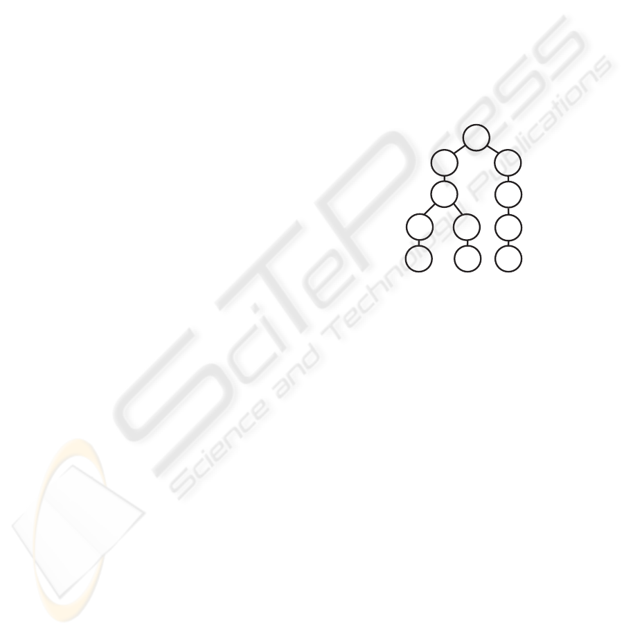
The special rec function approach is illustrated in
Fig.3 showing a random computer program created in
the initialization phase by employing the function set
F = {+, −, ∗, /, sin, cos, rec} and the terminal set
T = {1, −10, 10, −32, 775, 20, 807}, where instruc-
tion rec records the argument and passes it on un-
changed, and T consists of constants describing the
search space S from Fig. 1 (1, x
min
, x
max
, y
min
,
y
max
, ∆x and ∆y). The example program represents
the expression −10 · 1 + sin(775) and has a result of
−9.18. The five rec instructions, however, recorded
interim values −10, 1, −10, 775 and sin(775). The
interpretation of these is left to the individual’s eval-
uation function (for example, consecutive values can
be treated as coordinates of the hypercube corners).
rec rec
+
*
rec
-10
1
rec
sin
rec
775
Figure 3: Example program using the extended basic func-
tion set F and terminal set T of problem-specific constants.
The main problem of the basic approach is its slow
convergence speed. One possible improvement is the
use of automatically defined functions (ADFs) as de-
fined by (Koza, 1992), but this does not resolve the
problem. The convergence speed can be improved at
the expense of general applicability of functions and
terminals and this is what the next approach does.
3.3 GP Functions for Hypercube
Manipulation
Hypercube functions and terminals enable the GP to
manipulate D-dimensional hypercubes. Functions do
not handle scalar values as is the case with the basic
function set; rather they operate with and exchange
special objects that represent hypercubes.
A D-dimensional hypercube is uniquely defined by
at-least two opposite corner points (c
1
and c
2
) in a
D-dimensional hyper-space S (hyper-space S is actu-
ally the smallest hypercube encompassing all learn-
ing points in L). The function set and terminal set
must satisfy both the closure and the sufficiency cri-
teria. Additionally the instructions have to be highly
efficient in making the hypercube transformations.
CONSIDERATIONS FOR SELECTING FUNCTIONS AND TERMINALS IN GENETIC PROGRAMMING FOR
FAULT-DETECTION IN EMBEDDED SYSTEMS
145
A hypercube H
i
is a sub-space of the search space
S (H
i
⊆ S) and main idea is either to shrink and
re-position S into H
i
or “grow” the empty space ∅ to
become the final hypercube H
i
. Input to the computer
program can be any valid random hypercube S
′
(S
′
⊆
S).
Basic hypercube transformation functions and ter-
minals have mathematical origins and include (but are
not limited to):
union(A, B) function calculates the smallest hyper-
cube that includes both hypercubes A and B.
union is efficient and very simple to implement
function with results that quickly fill the whole
search space.
intersection(A, B) function returns the intersection
of hypercubes A and B. Common results is a small
hypercube or even a hyperpoint – latter may be use-
ful as an argument for other functions as it has zero
size and a fixed position in space.
scale
k
(A) function resizes the hypercube’s edges by
a constant pre-defined factor k. For different fac-
tors different functions must be defined.
move
i
(A, B) function must be defined for each di-
mension. It moves the hypercube A in the i − th
dimension by the length of hypercube B in this di-
mension: A
i
= A
i
+ ∆B
i
. Optionally a nega-
tive variant is possible, which can be invoked if
special criteria are met, e.g. if |B| > |A| the
A
i
= A
i
− ∆B
i
rule applies. This set of functions
allows for fine positioning of hypercube A.
comparison functions, e.g. <, ≤, = . . ., can be
based on the size of the compared hypercubes. Fur-
thermore, logical operators, e.g. if, can be de-
clared to give GP even more freedom in the search
for more robust solutions. They all return one of
the hypercube arguments; boolean cast is a simple
test of the non-emptyness of the hypercube.
(x) terminal is a hypercube with size 0, positioned at
a random hyperpoint (x) ∈ L.
S
′
terminal returns a random hypercube inside the
search space S. Of course each hypercube instance
is initialized differently every time it is used by a
newly created computer program, similarly to an
ephemeral constant. This allows great variability
in hypercubes offered by the terminal set.
S terminal returns S – the search space hypercube.
All these functions and terminals are universal –
they can be applied in any combination. One possible
hypercube GP setup is:
F = {union, intersection, scale
2
, scale
1/2
},
T = {S
′
, S}. (1)
GP equipped with (1) is able to find solutions simi-
lar to those found by GA, but more processing time
was needed to discover solutions of comparable qual-
ity. This is probably due to a fact that union and
intersection are binary functions and will produce a
perfect result only if both of its arguments are perfect.
This severe problem is addressed next.
3.4 GP: Extended Hypercube
Functions
The motivation is to create more robust versions of the
union and intersection operations. The perfect hy-
percube is (1) correctly positioned, and (2) has perfect
dimensions. If, for example, a binary union function
is to be made more robust, it should no longer be de-
pendable on correct position and size of both argu-
ments. Instead, a more relaxed transformation can be
introduced, which is based on complete correctness
of the first argument and for example, only on correct
size of the second argument. A call to union
′
(A, B)
will produce same result as union
′
(A, C), as long
|B| = |C|.
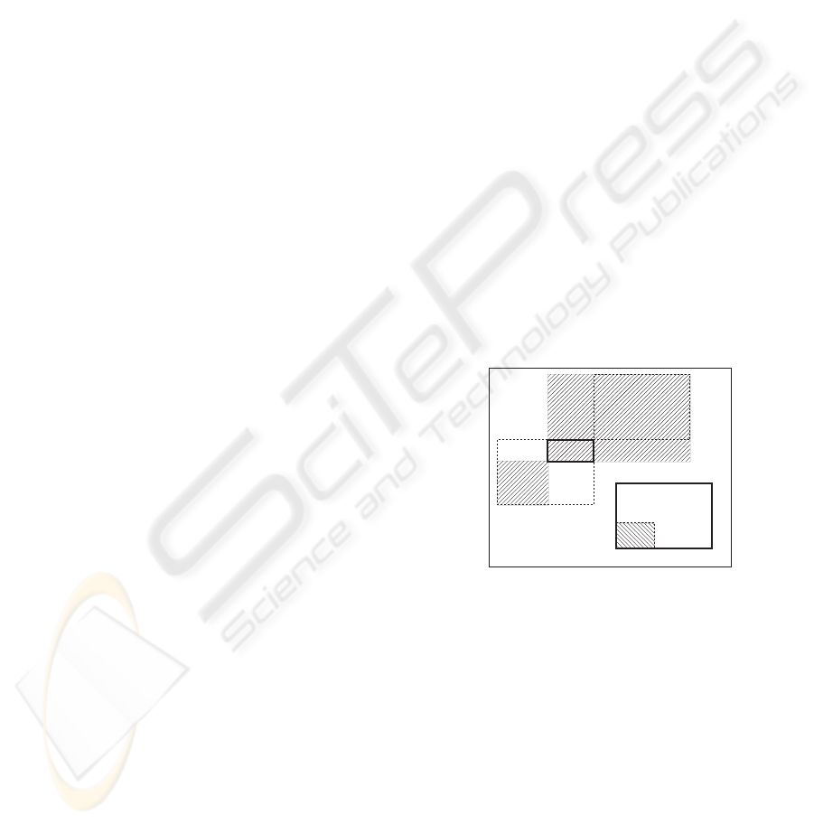
The inflate operation inflates the hypercube A to
“include” B as if B were positioned right next to A
and then union(A, B
′
) were called. This is depicted
in Fig. 4, where the original A and B hypercubes are
drawn with thick lines. The inflate(A, B) operation
aligns the b
1
corner of B with the a
2
of A.
x
max
x
min
y
max
y
min
S
a
2
a
1
inflate(A,B)
A
shrink(A,B)
scale(B,A)
b
2
b
1
B
Figure 4: Functions inf late, shrink and scale create
hatched hypercubes.
A similar operation is shrink, which aligns the
B’s b
2
corner with A’s a
2
and returns a hyper-
cube between b
′
1
and a
1
(Fig. 4). The chosen
two implementations are not commutative because
the result is always aligned according to the first hy-
percube: inflate(A, B) 6= inflate(B, A). How-
ever, the size of the resulting hypercubes is com-
mutative: |inflate(A, B)| = |inflate(B, A)| and
|shrink(A, B)| = |shrink(B, A)|.
Both functions can produce results outside of the
search space S. Such interim hypercubes may be
needed to produce final results within the whole S.
The final hypercube can be easily clipped to fit inside
S.
ICINCO 2006 - INTELLIGENT CONTROL SYSTEMS AND OPTIMIZATION
146

Next a powerful function that scales a hypercube
can be defined. Function scale(X, Y ) scales (inflates
or shrinks) the hypercube X; it effectively calls the
scale
k
(X), where k is calculated using:
k =
(
D
q
|Y |
|X|
if |X| 6= 0
1 otherwise.
Example in Fig. 4 shows the function scale(B, A),
which shrinks the hypercube B to approximately 40%
of its original size. The scale instruction is much
more flexible than the static scale
k
because it allows
GP to find a “perfect” scaling factor. The described
three functions accompanied by the two terminals S
and S
′
make the improved GP hypercube manipulat-
ing setup:
F = {inf late, shrink, scale},
T = {S
′
, S}. (2)
Table 1 shows the summary for 10 independent
runs of each method for the problem from Fig. 1.
Higher values are considered better although the over-
fitting limit is unknown. The GA used setup as de-
scribed in section 3.1, and GP was equipped with both
basic hypercube function set (1) and improved func-
tion set (2). Column 1 gives the average size of the
discovered hyperspace of invalid points S
−
and col-
umn 2 the biggest S
−
found by the respective method.
GP results come very close to GA’s (probably overfit-
ted) scores. Use of basic scalar functions and termi-
nals produced statistically inferior results when com-
pared to GA and GP using (1) or (2) and is not in-
cluded in this table.
Table 1: Summarized results for GA and GP equipped with
hypercube and improved hypercube manipulating functions
and terminals.
Method
Average(|S
−
|) Max(|S
−
|)
GA 9703 10051
GP using (1)
9251 9780
GP using (2)
9585 9808
4 CONCLUSION
The aim was to discover a general assortment of GP
functions and terminals in order to build programs for
fault-detection. The first step, presented here, was to
use GP as a machine learning algorithm to solve a typ-
ical problem in embedded system design; next is the
discovery of other GP functions and terminals which
would allow GP to discover ideal adaptive run-time
fault detection logic.
In many cases the analytical methods for space
partitioning and clustering are more appropriate than
evolutionary computation. For monitoring cells in
embedded control system design, however, EC is
quite suitable. The described GP functions and termi-
nals are able to define simplistic fault-detection rules.
Although the GAs are easier to implement and have
best convergence properties, GP is a promising op-
tion as it’s structure is self-evolving. The GA on the
contrary has a limited fixed solution structure.
The only advantage for using the basic scalar func-
tion and terminal set with GP lies in the simplicity
of use as they are available in all GP libraries. How-
ever, they are not efficient in producing hypercubes
directly. A better option would be to calculate opti-
mal partitioning of problem’s dimensions into inter-
vals, what effectively divides the search space into a
matrix of hypercubes. The hypercube manipulating
functions are a better choice: the improved set (2)
has better convergence properties than the basic set
(1). Another way to improve GP performance is to
search for partial solutions first by dividing the orig-
inal D-dimensional problem into a set of easier 2-D
problems.
The hypercubes are a simple and efficient strategy
for fault-detection. However, ambiguous points ex-
ist at hypercube boundaries and corners; such points
are close to the cluster of valid points. This also lim-
its the GP in discovering effective adaptive run-time
rules for fault detection as currently all results have to
be approved by a human. Further handling of detected
faults is out of scope of this paper.
ACKNOWLEDGEMENTS
This work was partially supported by the Ministry of
Higher Education, Science and Technology of Repub-
lic of Slovenia with the grant No. Z2-6398-0796.
REFERENCES
Banzhaf, W., Nordin, P., Keller, R., and Francone, F. (1998).
Genetic Programming – An Introduction. Morgan
Kaufmann, San Francisco.
Gagne, C. and Parizeau, M. (2006). Genericity in evolution-
ary computation software tools: Principles and case-
study. International Journal on Artificial Intelligence
Tools, 15(2):173–194.
Koza, J. (1992). Genetic Programming: On the Program-
ming of Computers by Natural Selection. MIT Press,
Cambridge, MA.
Schwefel, H.-P. (1987). Collective phenomena in evolu-
tionary systems. Preprints of the 31st Annual Meeting
of the International Society for General System Re-
search, Budapest, 2:1025–1033.
CONSIDERATIONS FOR SELECTING FUNCTIONS AND TERMINALS IN GENETIC PROGRAMMING FOR
FAULT-DETECTION IN EMBEDDED SYSTEMS
147
