ESTIMATION OF ROAD PROFILE USING SECOND ORDER
SLIDING MODE OBSERVER
A. Rabhi, N. K. M’Sirdi, M. Ouladsine
LSIS, CNRS UMR6168
Dom. Univ. St Jrme, Av Escadrille Normandie-Niemen 13397 Marseille France
L. Fridman
UNAM Dept of Control, Div. Electrical Engineering
Faculty of Engineering, Ciudad Universitaria, Universidad Nacional Autonoma de Mexico, 04510, Mexico, D.F., Mexico
Keywords:
First and second order sliding modes, Estimation of inputs, Road Profile, Robust nonlinear observers.
Abstract:
This paper presents an algorithm to estimate the road profile. This method is based on a robust observer
designed with a nominal dynamic model of vehicle. The estimation has been validated experimentally using a
trailer equipped with position sensors and acceleration sensors.
1 INTRODUCTION
For the purpose of road serviceability, surveillance
and road maintenance, several profilometers have
been developed. For instance, (Span) have proposed
a method based on direct measurements of the road
roughness. However, some drawbacks of this method
and some limitations of its capabilities have been
pointed out in (Meau1992). A profilometer is an in-
strument used to produce series of numbers related in
a well-defined way to the true profile (Span). How-
ever, this instrument produces biased and corrupted
measures. The Road and Bridges Central Labora-
tory in French (LCPC) has developed a Longitudinal
Profile Analyzer (LPA) (Legea1994). It is equipped
with a laser sensor to measure the elevation of road
profile. Other geometrical methods using many sen-
sors (distance sensor, accelerometers...) were also
developed (Gillespie1987). However, these meth-
ods depend directly on the sensors reliability and
cost. It is worthwhile to mention that these meth-
ods do not take into consideration the dynamic be-
havior of the vehicle. In a previous work, M’Sirdi
and al (M’Sirdi2005)(Im2003)(Rabhi2004) have pre-
sented an observer to estimate the road profile by
means of sliding mode observers designed from a dy-
namic modeling of the vehicle. But in the previous
method the vehicle rolling velocity is constant and
steering angle is assumed zero. For estimation of the
road profile, slope and inclination are also neglected.
The main contribution is here to extend this observer.
This paper is organized as follows: section 2 deals
with the vehicle description and modelling. The de-
sign of the second order sliding mode observer is pre-
sented in section 3. Some results about the states
observation and road profile estimation by means of
proposed method are presented in section 4. Finally,
some remarks and perspectives are given in a conclud-
ing section.
2 VEHICLE MODELING
In literature, many studies deal with vehicle mod-
elling (Kiencken2000)(Rabhi2004)(Ramirez1997).
The objective may be either confort analysis or
design or increase of safety and mailability of the
car. The system under consideration is a vehicle
represented as depicted in figure 1. This vehicle is
composed by a car body, four suspensions and four
wheels. The dynamic equations of the motion of the
vehicle body are obtained by applying the fundamen-
tal principle of mechanics. When considering the
vertical displacement along the z axis, the dynamic
of the system can be written as:
M ¨q + C ˙q + Kq = AU (1)
where (
.
q,
..
q) represent the velocities and accelerations
vector respectively. M ∈ R
7x7
is the inertia matrix,
C ∈ R
7x7
is related to the damping effects, K ∈ R
7x7
is the springs stiffness vector (see Figure 1). The car
body is assumed rigid. q ∈ R
7
is the coordinates
vector defined by:
q = [z
1
, z
2
, z
3
, z
4
, z, θ, φ] (2)
531
Rabhi A., K. M’Sirdi N., Ouladsine M. and Fridman L. (2006).
ESTIMATION OF ROAD PROFILE USING SECOND ORDER SLIDING MODE OBSERVER.
In Proceedings of the Third International Conference on Informatics in Control, Automation and Robotics, pages 531-534
DOI: 10.5220/0001215905310534
Copyright
c
 SciTePress

The matrix M, C, K and A are defined in
(Rabhi2004). z
i
i = 1..4 is the displacement of the
wheel i. z, θ and φ represent the displacements of the
vehicle body, roll angle, and pitch angle respectively.
Figure 1: Vehicle Model.
K
i
: are the suspension spring stiffness [N/m],
B
i
: are the suspension damping [N/m/s],
K
ri
: are the tire spring stiffness [N/m],
B
ri
: are the tire spring damping [N/m/s],
U = [
u
1
u
2
u
3
u
4
]
T
is the vector of un-
known inputs which characterizes the road profile.
The vertical dynamical model 1 can be written in
the state form as follows:





x
1
= q
˙x
1
= x
2
˙x
2
= ¨x
1
= ¨q = M
−1
(−Cx
2
− Kx
1
+ AU)
y = x
1
.
(3)
where the state vector x = (x
1
, x
2
)
T
= (q,
.
q)
T
, and
y = q (y ∈ R
7
) is the vector of measured outputs of
the system.
y = [
z
1
z
2
z
3
z
4
z θ φ
]
T
(4)

˙x
1
= x
2
˙x
2
= f(x
1
, x
2
) + ξ
. (5)
with f(x
1
, x
2
) = M
−1
(−Cx
2
− Kx
1
). The un-
known input component isξ = M
−1
AU
3 ESTIMATION OF THE ROAD
PROFILE
In order to estimate the state vector x and to deduce
the unknown inputs vector U, we propose the follow-
ing second order sliding mode observer (Davila2004):
˙
ˆx
1
= ˆx
2
+ z
1
˙
ˆx
2
= f(t, x
1
, ˆx
2
) + z
2
(6)
where ˆx
1
and ˆx
2
are the state estimations, and the
correction variables z
1
and z
2
are calculated by the
super-twisting algorithm
z
1
= λ|x
1
− ˆx
1
|
1/2
sign(x
1
− ˆx
1
)
z
2
= α sign(x
1
− ˆx
1
).
(7)
The initial moment ˆx
1
= x
1
and ˆx
2
= 0, are taken to
ensures observer convergence. We assume x
1
avail-
able for measurement and we propose the following
sliding mode observer:
.
bx
1
= bx
2
+ λ
p
|x
1
− bx
1
|sign(x
1
− bx
1
) (8)
.
bx
2
= f(x
1
, ˆx
2
) + αsign(x
1
− bx
1
) (9)
where bx
i
represent the observed state vector and α, β
and λ are the observer gains.
It i important to note that in a first step, input effects
on the dynamic are rejected by the proposed observer
like a perturbation. Taking ˜x
1
= x
1
− ˆx
1
and ˜x
2
=
x
2
− ˆx
2
we obtain the equations for the estimation
error dynamics
˙
˜x
1
= ˜x
2
− λ|˜x
1
|
1/2
sign(˜x
1
)
˙
˜x
2
= F (x
1
, x
2
, ˆx
2
) − α sign(˜x
1
)
(10)
Let us recall that
F (t, x
1
, x
2
, ˆx
2
) = f (t, x
1
, x
2
) − f (t, x
1
, ˆx
2
) + ξ(t, x
1
, x
2
)
In our case, the system states are bounded, then the
existence of a constant bound f
+
is ensured such that
|F (x
1
, x
2
, ˆx
2
)| < f
+
(11)
holds for any possible t, x
1
, x
2
and |ˆx
2
| ≤ 2v
max
.
v
max
and x
max
are defined such that ∀t ∈ R
+
∀x
2
, x
1
|x
2
| ≤ v
max
and x
1
≤ x
max
The state boundedness is true, because the mechan-
ical system (5) is BIBS stable, and the control input
u is bounded. The maximal possible acceleration in
the system is a priori known and it coincides with the
bound f
+
. In order to define the bound f
+
let us
consider the system physical properties. We have: -
m
I ≤ M ≤ mI - cI ≤ M ≤ cI - kI ≤ M ≤ kI
where m, c and k are the minimal respective eigen-
values and m, c and k the maximal ones. Then we
obtain max(M
−1
) =
1
m
I and f
+
can be written as
f
+
=
1
m
(cv
max
+ kx
max
) Let α and λ satisfy the fol-
lowing inequalities, where p is some chosen constant,
0 < p < 1
α > f
+
,
λ >
q
2
α−f
+
(α+f
+
)(1+p)
(1−p)
,
(12)
The previous observers ensures that in finite time we
have ex
2
= 0 then
˙
˜x
2
= f(x
1
, x
2
) − f(x
1
, ˆx
2
) + ξ − z
2
= 0 (13)
Let us take a low pass filtering of z
2
which is defined
in equation 6 and 7, then we obtain in the mean aver-
age:
ξ = z
2
(14)
Note that z
2
is the filtered version of z
2
. In order to
estimate the elements u
i
i = 1...4 of the unknown
input vector U and according 2 we can write
ζ
1
= A
11
U
u
+ B
11
˙
U
u
ICINCO 2006 - ROBOTICS AND AUTOMATION
532

with ζ = [
ζ
1
0 0 0
]
T
, and the matrices A
11
and B
11
given in (Rabhi2004). For i = 1..4 we have
ζ
1i
= a
ii
u
i
+ b
ii
.
u
i
(15)
where a
ii
and b
ii
are respectively the elements of A
11
et B
11
. To solve this system we can take an approach
simpler that the one in (Im2003) which uses a stan-
dard observer.
We can write:

.
u
i
= g(u
i
, ζ
1i
)
ζ
1i
= h(u
i
)
(16)
with:
g(u
i
, ζ
1i
) =
1
b
ii
(−a
ii
u
i
+ ζ
1i
) (17)
The observer proposed here is the:
.
bx
i
= f(bx
i
, ey
i
) + λ
i
(y
i
− by
i
) (18)
Let us not the the observation error: eu
i
= u
i
− bu
i
The observation error dynamics is then obtained from
equation (16) and (18).
.
eu
i
= g(eu
i
, ζ
1i
) + λ
i
(
e
ζ
1i
) The
convergence is proved by the following Lyapunov
candidate function:V
i
=
1
2
eu
2
i
The time derivative of
V is then:
.
V
i
= eu
i
.
eu
i
from 17, we obtain:
.
V
i
= eu
i

1
b
ii
(−a
ii
eu
i
+
e
ζ
1i
) − λ
i
(
e
ζ
1i
)

(19)
and then as ζ
1i
is measured or reconstructured by a
observer we choose: λ
i
=
1
b
ii
, on
.
V
i
< 0,
4 EXPERIMENTAL RESULTS
In this section, we present some experimental re-
sults to validate our approach. Several trials have
been done with a vehicle (P406 of LCPC) equipped
with different sensors. Some tests were carried out
at the Road and Bridges Central Laboratory (LCPC)
test track with an instrumented car towing two LPA
trailers. Measures have been acquired with the ve-
hicle rolling at several speeds. The signal measured
by a Longitudinal Profile Analyzer (LPA) constitutes
in this experiment our reference profile. The figure
2 shows the vehicle speed variations. The Figure 3
shows clearly that the estimated displacements of the
four wheels converge quickly to the measured ones.
we present the roll angle and the pitch angle.
A good reconstruction of state enables the estima-
tion of the unknown inputs of the system. Figure 5
presents both the measured road profile (coming from
LPA instrument) and the estimated one. We can then
observe that the estimated values are quite close the
true ones.
Figure 2: Longitudinal velocity of the vehicle.
Figure 3: Displacements of wheels: estimated and mea-
sured.
5 CONCLUSION
In this paper, we present enhancement of the previ-
ously proposed method to estimate the road profile
elevation based on second-order sliding-mode. The fi-
nite time convergence of the observer is proved. The
gains of the proposed observer are chosen very eas-
ily ignoring the system parameters. This observer is
compared, using experimental data. This observer is
better than the previous one in convergence and do not
assume the velocity constant. This is due to robust-
ness of the second order observer which allows better
rejection of perturbation and then a better reconstruc-
tion of the unknown inputs. The latter reconstruction
has been also enhanced.
The estimation scheme build up using a Second Or-
der Sliding Mode observers has been tested on ex-
perimental data (acquired with a P406 vehicle) and
shown to be very efficient. The actual results prove
effectiveness and robustness of the proposed method.
In our further investigations the estimations produced
on line will be used to define a predictive control to
enhance the safety.
ACKNOWLEDGEMENTS
J. Davila and L. Fridman gratefully acknowledge the
financial support of the Mexican CONACyT, and of
the Programa de Apoyo a Proyectos de Investigacion
e Innovacion Tecnolgica (PAPIIT) UNAM.
This work has been done in a collaboration man-
aged by members of the LSIS inside the GTAA (re-
search group supported by the CNRS).
Many thanks are addressed by the authors to the
LCPC of Nantes for experimental data and the trials
with their vehicle Peugeot 406.
ESTIMATION OF ROAD PROFILE USING SECOND ORDER SLIDING MODE OBSERVER
533

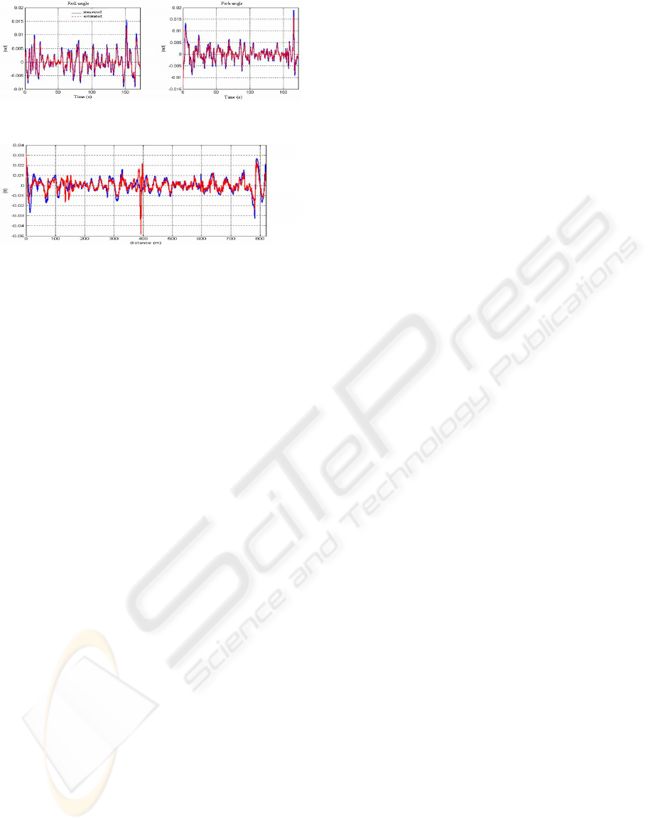
Figure 4: Estimation of the roll angle and the pich angle.
Figure 5: Comparison between observers approach and
LPA profile.
REFERENCES
E.B. Spangler and W.J. Kelly, GMR Road Profilometer
Method for Measuring Road Profile.
Meau- Fuh ”Pong, The Development of an Extensive-
Range Dynamic Road Profile and Roughness Measur-
ing System”, May 1992.
Vincent Legea ”Localisation et d
´
etection des d
´
efauts d’uni
dans le signal APL ”, Bulletin de liason du labora-
toire Central des Ponts et Chauss
´
ees, n
◦
192, juillet
ao
ˆ
ut 1994.
T.D Gillespie and al., Methodology for R oad Roughness
Profiling and Rut Depth Measurement, Federal High-
way Administration Report FHWA/RD-87042, 1987
50 p.
H.Imine,N.K. M’Sirdi, Y.Delanne, Adaptive Observers and
Astimation of the Road Profile, SAE Word Congress,
vehicle dynamics and simulation Mars 2003, pp. 175-
180, Detroit, Michigan.
A. Rabhi, Imine, N. M’ Sirdi and Y. Delanne. Observers
With Unknown Inputs to Estimate Contact Forces and
Road Profile AVCS’04 International Conference on
Advances in Vehicle Control and Safety Genova Italy,
Oct28-31.
U. Kiencken, L. Nielsen. Automotive Control Systems.
Springer, Berlin, 2000.
A. Rabhi, N. K. M’sirdi, N. Zbiri and Y. Delanne.
Mod
´
elisation pour l’estimation de l’
´
etat et des forces
d’Interaction V
´
ehicule-Route, CIFA2004.
R. Ramirez-Mendoza. Sur la mod
´
elisation et la commande
des v
´
ehicules automobiles. PHD thesis Institut Na-
tional Polytechnique de Grenoble, Laboratoire d Au-
tomatique de Grenoble 1997.
J.P. Barbot, M. Djemai, and T. Boukhobza. Sliding Mode
Observers; in Sliding Mode Control in Engineering,
ser.Control Engineering, no. 11, W. Perruquetti and
J.P. Barbot, Marcel Dekker: New York, 2002, pp. 103-
130.
G. Bartolini, A. Pisano, E. Punta, and E. Usai. ”A survey
of applications of second-order sliding mode control
to mechanical systems”, International Journal of Con-
trol, vol. 76, 2003, pp. 875-892.
A. Pisano, and E. Usai, ”Output-feedback control of an
underwater vehicle prototype by higher-order sliding
modes ”, Automatica, vol. 40, 2004, pp. 1525-1531.
J. Davila and L. Fridman. “Observation and Identifica-
tion of Mechanical Systems via Second Order Slid-
ing Modes”, 8th. International Workshop on Variable
Structure Systems,September 2004, Espana
A. Levant, ”Sliding order and sliding accuracy in sliding
mode control,” International Journal of Control, vol.
58, 1993, pp 1247-1263.
J. Alvarez, Y. Orlov, and L. Acho, ”An invariance principle
for discontinuous dynamic systems with application
to a coulomb friction oscillator”, Journal of Dynamic
Systems, Measurement, and Control, vol. 122, 2000,
pp 687-690.
Y.B. Shtessel, I.A. Shkolnikov, and M.D.J. Brown, ”An as-
ymptotic second-order smooth sliding mode control”,
Asian Journal of Control, vol. 5(4), 2003, pp 498-504.
A. Levant, ”Robust exact differentiation via sliding mode
technique”, Automatica, vol. 34(3), 1998, pp 379-384.
A.F. Filippov, Differential Equations with Discontin-
uous Right-hand Sides, Dordrecht, The Nether-
lands:Kluwer Academic Publishers; 1988.
V. Utkin, J. Guldner, J. Shi, Sliding Mode Control in
Electromechanical Systems, London, UK:Taylor &
Francis; 1999.
N. M’sirdi, Y. Delanne, A. Rabhi “Observateurs robustes
et estimations de forces de contact, reconstitution du
profil de chauss
´
ees”, in: Journ
´
ees ADV: Automatique
et Diagnostic pour le V
´
ehicule, ADV 2005, Marseille,
France, 2005
ICINCO 2006 - ROBOTICS AND AUTOMATION
534