
REACTIVE SIMULATION FOR REAL-TIME OBSTACLE
AVOIDANCE
Mariolino De Cecco
Dep. Mech Struct Eng, University of Trento, Via Mesiano 77, Trento, Italy
Enrico Marcuzzi, Luca Baglivo, Mirco Zaccariotto
CISAS, Centre of Studies and Activities for Space, Via Venezia 1, 35131 Padova, Italy
Keywords: AGV, reactive simulation, obstacle avoidance.
Abstract: This paper provides a new approach to the dynamic path planning and obstacle avoidance in unknown and
dynamic environments. The system is based on the interaction between four different modules: the Path
Planner, the Graph which memorizes all the local target, the “Sentinel”, and the module which computes the
Reactive Simulation every time an obstacle is detected along the path. The Reactive Simulation takes in
account the kinematics model of the vehicle and the actual state conditions to make a real-time simulation in
order to predict the trajectory of the differential drive robot that would allow the safe reaching of the local
target.
1 INTRODUCTION
The main aspects in the field of Autonomous Guided
Vehicles are the safety of motion planning and
accurate pose measurement. Both of these aspects
are still challenging problems.
Improving the degree of system autonomy
makes possible to use AGV in unknown and
dynamic environments, where the main problem is
to avoid obstacles and trap situations. Main aspects
which have to be taken into consideration are
dynamic obstacles, accurate relative pose estimation,
kinematics and dynamical parameters variations.
Past studies concerning obstacle avoidance
(Khatib, 1986; Koren, Borentein, 1991) were based
on potential fields where obstacles exert repulsive
forces, while the target applies an attractive force to
the robot. A resultant force vector is calculated for a
given robot position and it gives the current motion
direction. These methods have strong limitations in
approaching doors, U-shape obstacles and in
avoiding trap situations. Virtual Force Histogram
(VFH) was developed to improve and make the
potential field method more robust: it uses a two-
dimensional Cartesian histogram grid as a world
model to reduce sensors data and to compute the
desired control motion for the vehicle (Borentein,
Koren, 1991; Ulrich, Borentein, 1998; . Ulrich,
Borentein, 2000).
Based on potential field methods, other studies
were focused on a dynamical building of figure
(Dynamic Force Fields) where the magnitude in
each point can be seen as proportional to the
probability of collision at that point (Planas).
All these methods, when operating in unknown
environment cannot really solve trap-situations and
can’t find an optimal path (it can only be found
when complete environmental information is given).
In order to search for optimality it is possible to
build a map during motion with the application of
Kalman filter (Nebot, Durrant-Whyte, 1999), but
this can become useless in very dynamic
environments, like factories or ports with a lot of
vehicles in motion, thus wasting computational time.
To cope with dynamic environments, sensor-
based motion generation techniques were developed:
environmental changes or moving obstacles detected
by sensors imply a “reactive path planning”,
adapting robot motions to every new event, and
sensorial measures are used to create a local model
of the environment exploited to drive the robot
safely, also in dense and cluttered scenarios
(Minguez,, Montano, 2005).
A different approach (Kelly, Nagy, 2002) is a
complete trajectory generation: based on real-time
128
De Cecco M., Marcuzzi E., Baglivo L. and Zaccariotto M. (2006).
REACTIVE SIMULATION FOR REAL-TIME OBSTACLE AVOIDANCE.
In Proceedings of the Third International Conference on Informatics in Control, Automation and Robotics, pages 128-135
DOI: 10.5220/0001216501280135
Copyright
c
SciTePress
perceptual information, a feasible nonholonomic
motions plan (from a given initial posture to a given
final posture) is generated using a parametric
representation. With this approach the main problem
is the computational time, and the existence of a
trajectory which satisfies all the boundaries and
conditions, namely the solution of a constrained
optimization problem. But this approach doesn’t
take into account the model of the vehicle and so
possible changes in kinematics and dynamical
parameters.
In fact the environment could change, as well as
kinematics parameters, affecting vehicle’s path.
This second aspect is usually not taken into account
in path planning and obstacle avoidance.
In recent times simulation techniques have been
applied to real-time systems optimization (De
Cecco, 2005).
In this paper we describe a reactive simulation
starting every time that a new target position is
planned during motion due to the detection of an
obstacle: if the output of the simulation is safe
obstacle avoidance the robot continues smoothly its
path, otherwise it stops to avoid dangerous collisions
and to plan a safe path. The output is a more robust
real time obstacle avoidance algorithm that would
allow navigation in unknown and dynamically
changing environment.
An important advantage of this approach is that
the use of a model for simulation permits to estimate
on-line the kinematics parameters and this allows to
take into account parametric variations like different
diameters of wheels, inertia of masses, etc, that
could affect sensibly vehicle’s motion (De Cecco,
2002).
The algorithm was implemented on an
autonomous vehicle with differential drive
kinematics (Figure 2). A PXI (National Instruments)
with an embedded real-time operating system
(RTOS) was used to control the robot and
implement the Reactive Simulation.
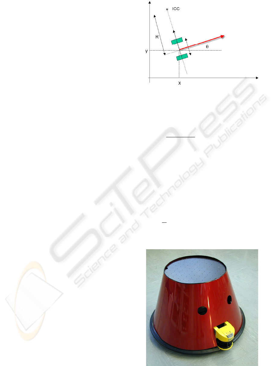
2 KINEMATICS MODEL
The vehicle used in the experiment has a differential
drive kinematics (Figure 1):
δ
b
Figure 1: Differential drive kinematics.
The discrete form of the Inertial-Odometric
navigation equations is the following:
⎪
⎪
⎩
⎪
⎪
⎨
⎧
+=
+=
+
−
=
−
−
−
1
1
1
)sin(
)cos(
)(
kckkk
kckkk
kc
lkrk
k
yTvy
xTvx
T
b
vv
δ
δ
δδ
(1)
where b is the distance between the centers of the
two wheels,
rk
v and
lk
v are the linear velocities of
right wheel and left wheel,
k
v is the velocity of
vehicle relative to the mid-point of axis b:
)(*
2
1
lkrkk
vvv += (2)
c
T is the period of the task which estimates the
pose.
Figure 2: The prototype of AGV used in the experiment.
REACTIVE SIMULATION FOR REAL-TIME OBSTACLE AVOIDANCE
129
3 SIMULATION OPTIMIZATION
Kinematics parameters were measured and then
optimized by minimizing a function cost which
considers the pose estimated by odometric and the
one estimated by the reference infrared triangulation
system (De Cecco, 2000).
As regards the CC motor, it was used this model:
- Electrical part:
)(
)(
)()( tK
dt
tdi
LtRitV
a
ω
Φ
++= (3)
where R is the resistance and L is the inductance
of electric circuit,
Φ
K
is the constant of torque,
a
V is the input voltage,
ω
is the angular velocity,
- Mechanical part:
)()()()( tBtJtiKt
m
ω
ω
τ
+==
Φ
(4)
where
m
τ
is the motor torque, J is the rotor
inertia,
B
is the viscous friction.
Combining the two parts:
R
s
L +
1
R
s
L +
1
B
s
J
+
1
B
s
J
+
1
Φ
K
Φ
K
Φ
K
Φ
K
+
-
a
V
i
τ
ω
Figure 3: Scheme of CC motor.
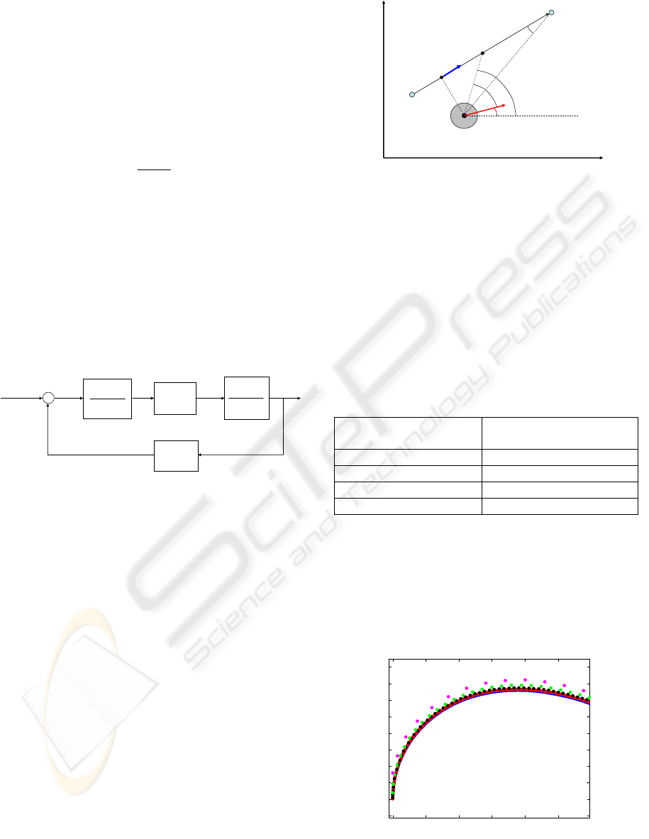
Concerning to Figure 4, the trajectory is tracking
projecting the center of vehicle on the segment P1P2
(where P1 is the target just reached and P2 is the
new target planned) obtaining Pp, computing the
point Pi:
120
LdPpPi += (5)
where
0
d is distance between Pp and Pi, and
imposing the angular velocity of the vehicle
according to:
δ
ω
k=
(6)
X
Y
P1
P2
Pp
δ
Pi
β
L12
θ
Pr
φ
Figure 4: Scheme of trajectory tracking.
The step of integration in simulation was chosen
as a compromise between computational time (it is a
real time simulation) and accuracy of trajectory.
Errors between simulations with a step of integration
of 1 ms and simulations with increasing steps are
shown in Table 1, which summarizes a set of tests
with different velocities and trajectories, and with
different initial heading with respect to the point to
reach:
Table 1: Maximum simulated errors increasing step of
integration in simulation.
Step of integration Maximum simulated
error
25 ms 8 mm
50 ms 16 mm
100 ms 32 mm
200 ms 61 mm
A maximum error of 16 mm enters in boundaries
of safe robot motion, on the contrary a step of
integration of 100 ms would be too inaccurate. A
good compromise was considered a maximum step
of 50 ms. In Figure 5 it is clear as the simulated
trajectories get worse increasing the step of
integration.
0 0.2 0.4 0. 6 0. 8 1
-0.1
0
0.1
0.2
0.3
0.4
0.5
0.6
0.7
0.8
Simul ated traject ories
X, [m ]
Y, [m]
Figure 5: a detail of simulated trajectories with increasing
steps of integration: 1 ms (blue), 25 ms (red), 50 ms
(black), 100 ms (green), 200 ms (pink).
ICINCO 2006 - ROBOTICS AND AUTOMATION
130
The computational time of Reactive Simulation
is a very important aspect in real time applications.
It depends on various influence quantities: actual
velocity of vehicle, length of the trajectory that has
to be simulated, initial pose of vehicle, step of
integration. Table 2 shows computational times of
Reactive Simulation: a trajectory of 2 m at the
velocity of 0.4 m/s was simulated with different
steps of integration, and for every step with different
heading with respect to the point to reach.
Table 2: Computational time of Reactive Simulation:
every time is the mean of simulations with different
heading with respect to the point to reach.
Step of integration Mean Time
10 ms 69 ms
20 ms 36 ms
30 ms 25 ms
40 ms 19 ms
50 ms 16 ms
It is clear as faster simulation has to be preferred
for real time applications and so a step of integration
of 50 ms was chosen
4 DYNAMICAL PATH PLANNING
The Planner makes a dynamical path planning to
reach the goal with no a priori information about the
environment. The only information are the initial
position of the vehicle and the final target position.
Planner searches for open spaces and for doors: the
so called “openings”. Dynamically the planner
makes a representation of the environment based on
a graph, which memorizes all the openings. In this
way the problem of dead-ends can be solved: when
no opening is found, the vehicle rotates on its own
axes by 180° degrees, then it searches again and if
actual openings are yet memorised in the graph, the
planner understands that it is probably in a dead-end.
So based on the openings memorised in the graph,
the new path is planned: the vehicle goes to a point
memorised but not yet visited, selected by A* search
algorithm . A* search is a common algorithm based
on a heuristic function which permits to make a local
optimal choose (because any map of the
environment is available) (Chestnutt, Kuffner,
Nishiwaki, Kagami, 2003; Stentz, 1994).
5 THE MEASUREMENT SYSTEM
The vehicle used in experiment is equipped with an
encoder for every wheel, and a laser range finder.
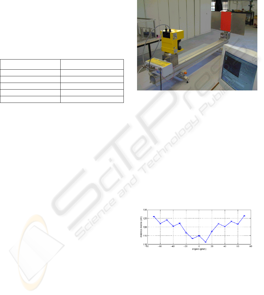
Figure 6: Experimental apparatus used for laser
characterisation.
In order to characterise the laser range finder it
has been mounted on a calibration setup (see Figure
6 ) composed of a bar for optical alignment, a panel
hinged in the axis orthogonal to the bar, whose
rotation is measured with an incremental encoder
with 14400 ppr.
By means of the above system it was first
characterised the noise standard deviation that come
out to be about 4 mm, then the effect of the
following influence parameters on laser accuracy:
temperature drift, distance, surface colour, surface
material, angle of incidence with respect to the
object.
Figure 7: Measurement as a function of the incidence
angle. Measurements taken with the target at fixed
distance of 115 cm with the apparatus of Figure 6.
Above all influence quantities the angle of
incidence plays a major role in degrading the
measurement accuracy. The effect of the incidence
angle over range estimation is shown in Figure 7. It
is evident that uncertainties of about 200 mm can
arise only because of rotation or perspective effects.
REACTIVE SIMULATION FOR REAL-TIME OBSTACLE AVOIDANCE
131
Uncertainty of range data was taken to apply a
margin to the output of the Reactive Simulation.
The above characterisation is important also
because laser scan data are now starting to be used
for pose estimation (De Cecco, 2006).
6 REACTIVE SIMULATION
Reactive Simulation is an algorithm based on the
vehicle’s model which compute a simulation of the
trajectory to the local target.
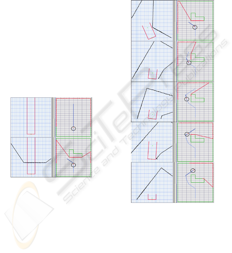
This is the logical scheme of interaction between
modules (as it can be seen in Figure 9):
1. “Planner” chooses a local target, and vehicle
moves towards it (see first frame of Figure 8a,
where a simulation of obstacle avoidance is
shown).
2. “Sentinel” checks environment to detect moving
obstacles or something like these in robot’s
trajectory (in second frame of Figure 8a, on the
left an obstacle detected by the Sentinel).
Figure 8a: Example of simulation of obstacle avoidance.
On the right side is shown the trajectory of vehicle. On
the left side it’s shown the Sentinel, which checks a virtual
corridor from the actual position of vehicle to the local
target to detect any obstacle, as happens in second frame,
where an obstacle suddenly appears.
3. If obstacles are detected, Sentinel alerts the
Planner which find a new local target (in second
frame of Figure 8a, on the right the new local
target planned).
4. Then Reactive Simulation starts, simulates the
trajectory to cover to reach the actual local target,
and communicates to Planner if the computed
trajectory crashes into some obstacles or not (see
Figure 12c and 12d).
5. Finally planner decides to reach or not the local
target. In the first case vehicle continues
smoothly its path, otherwise it stops to avoid
dangerous collision and to plan a safe path (in the
first frame of Figure 8b, the vehicle continues to
move towards the local target).
Figure 8b: Example of simulation of obstacle avoidance.
By this way, and integrating the reactive
simulation with an on-line identification parameters
algorithm, it could be possible to take into account
variations in kinematics parameters, for example
diameters of wheels, inertia of masses, etc, that
could affect sensibly vehicle’s motion.
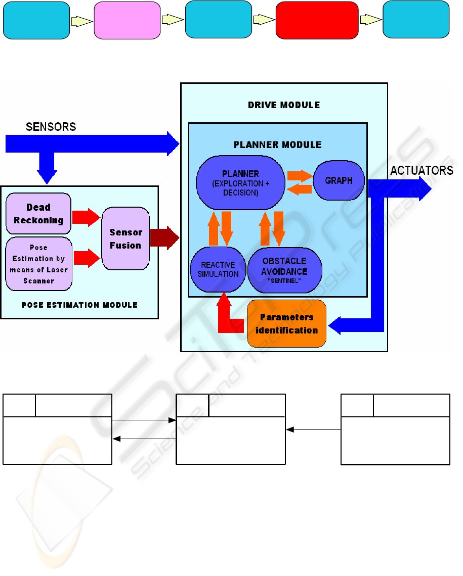
A complete scheme of the Drive Module is
shown in Figure 10.
ICINCO 2006 - ROBOTICS AND AUTOMATION
132
PLANNE R
REA CTI VE
SIMULATI ON
SENTI NEL
PLA NNER PLANNE R
1. 2. 3. 4. 5.
Figure 9: Logical scheme of interaction between different modules.
Figure 10: Complete scheme of Drive Module, and its interaction with Sensors Fusion Algorithm and on-line Parameters
Identification Algorithm.
Scanning
Tc=15
ms
TAS K 1
[High Priority]
ODOMETRIC POSE
ESTIMATION
-trajectory tracking
Tc=6
ms
TAS K 2
[Critical Priority]
COMMUNICATION
WITH LASER PLS
Tc=30
ms
TAS K 3
[Normal Priority]
PATH PLANNER
-planning
-obstacle avoidance
-Reactive Simulation
Pose
Setpoint
Figure 11: Scheme of the three main tasks.
7 REAL-TIME
IMPLEMENTATION
Reactive Simulation has been implemented in real-
time applications using the prototype of autonomous
vehicle. It is equipped with a 333 MHz PXI
(National Instruments) with an embedded real-time
operating system (RTOS). The software has three
main tasks (see Figure 11):
• TASK 1 which estimates the pose with data
from odometers sensors and executes the
trajectory tracking
• TASK 2 of communication with laser
• TASK 3 which makes the path planning,
obstacle avoidance and Reactive Simulation.
The priority (static-priority) of the tasks was
initially assigned according to rate monotonic
algorithm which assign the priority of each task
REACTIVE SIMULATION FOR REAL-TIME OBSTACLE AVOIDANCE
133
according to its period, so that the shorter the period
the higher the priority.
In order of priority:
• TASK 2 has a worst-case execution time of 2-3
ms (except when a scan is received), a period of
6 ms, and so has critical priority
• TASK 1 has a worst-case execution time of 4-5
ms, a period of 15 ms, and so has high priority
• TASK 3 has a worst-case execution time of 10-
12 ms, a period of 30 ms, and so has normal
priority.
But in this way when a scan from laser was
received (every 200 ms), the TASK 2 has to make a
lot of calculates utilizing CPU for about 16 ms and
so getting worse the pose estimation, which is the
main aspect. Therefore priority of TASK 1 is now
critical, and priority of TASK 2 is high.
The Reactive Simulation algorithm is part of
Planner Module (TASK 3), and so has normal
priority.
8 EXPERIMENTAL
VERIFICATION
The prototype used in the experiments is a
differential drive robot. It has a diameter of 1.05 m,
height is 0.9 m and maximum velocity is about 2.5
m/s.
Many trajectories were tested with sudden and
dynamic obstacles, in which were taken into account
the standard deviation of laser’s scans and the linear
and angular velocities of the vehicle when the scans
were received to perform a safe robot motion. In
fact, the trajectory is planned based on scans closer
to vehicle respect to the received scans (see pink line
in Figure 12c and 12d which represents the closer
scan). The distance between the received scan and
“the safe” one depends on actual linear and angular
velocities of the vehicle.
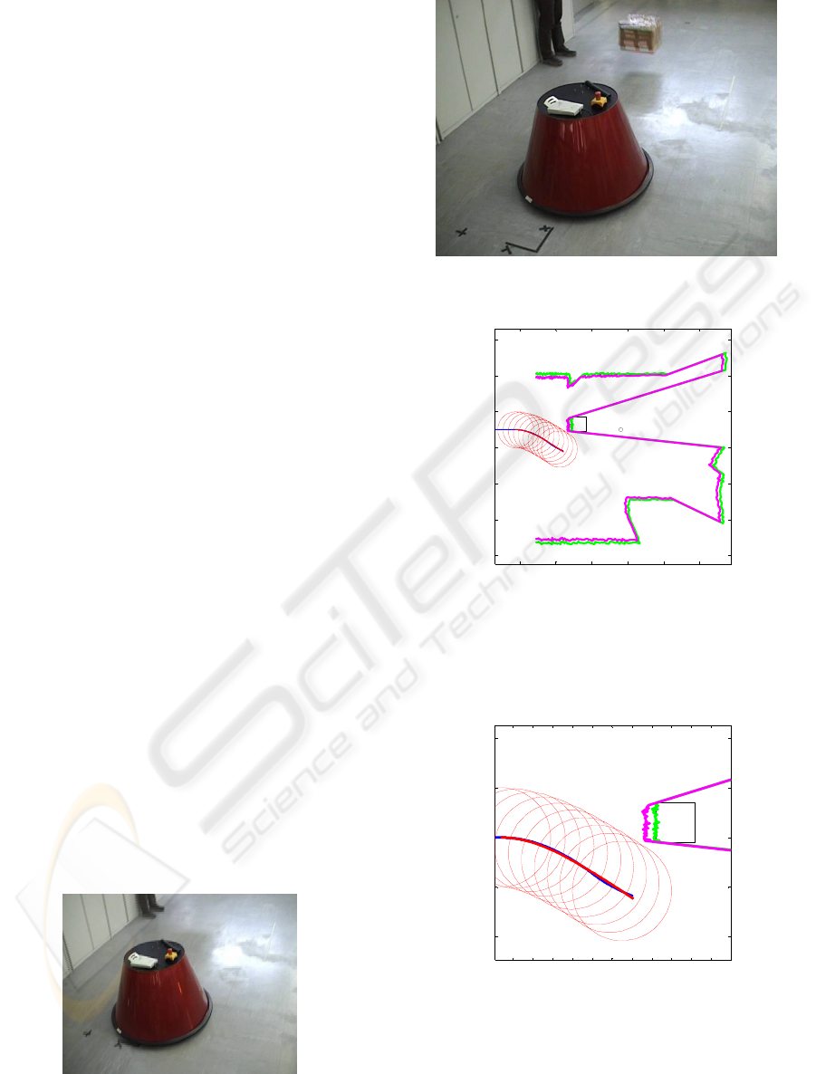
An example of obstacle avoidance is shown in
Figure 12.
Figure 12a: Example of obstacle avoidance with Reactive
Simulation: the vehicle starts to move toward target.
Figure 12b: an obstacle suddenly appears.
3 4 5 6 7 8
-2
-1
0
1
2
3
4
X [ m]
Y [m]
Figure 12c: a new local target was planned and Reactive
Simulation computes the trajectory (the red lines). The
green line is the received scan and the pink one is the
calculated closer scan.
3 3.2 3. 4 3.6 3.8 4 4.2 4.4 4.6 4.8 5
0.5
1
1.5
2
2.5
X [ m]
Y [m]
Figure 12d: a detail of Reactive Simulation where the blue
line is the real trajectory made by vehicle after the
Reactive Simulation.
ICINCO 2006 - ROBOTICS AND AUTOMATION
134
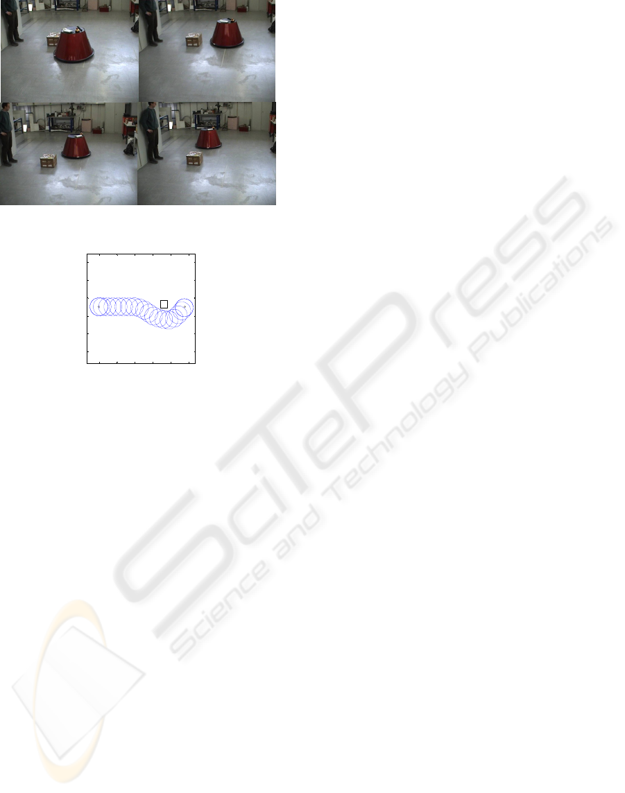
Figure 12e: safe robot motion to the target.
1 2 3 4 5 6
-1
0
1
2
3
4
X [ m]
Y [m]
Figure 12f: entire real trajectory.
9 CONCLUSIONS
This paper presents a novel technique called
“Reactive Simulation” for real-time obstacle
avoidance. A vehicle’s trajectory simulation starts
every time a new local target is planned due to the
detection of an obstacle. It was verified that 50 ms
integration step permits a fast simulation and the
maximum error enters in boundaries of safe robot
motion. The algorithm was successfully tested on a
vehicle in real-time applications, where an important
aspect is the correct execution of the tasks which
have to communicate with sensors, to estimate the
pose and to plan a safe path.
REFERENCES
Oussama Khatib, 1986, Real-Time Obstacle Avoidance
for Manipulators and Mobile Robot, in: The
International Journal of Robotics Research, Vol. 5,
No 1.
Y. Koren, J. Borentein, 1991, Potential Field Methods and
their Inherent Limitations for Mobile Robot
Navigation, in: Proceedings of the IEEE conference on
Robotics and automation, Sacramento, California,
April 7-12, pp 1398-1404.
J. Borentein, Y. Koren, 1991, The Vector Field histogram
– fast obstacle avoidance for mobile robot, in: IEEE
Journal of Robotics and Automation, Vol 7, No 3,
June, pp. 278-288.
Minguez, J., Montano, L., 2005. Sensor-based motion
generation in unknown, dynamic and troublesome
scenarios,in: Robotics and Automation Systems. 52, pp
290-311.
Planas R.M., Fuertes J.M., Martinez A.B.,Qualitative
Approach for Mobile Robot Path Planning based on
Potential Field Methods, Automatic Control Dept.
Technical University of Catalonia.
E.M. Nebot, H. Durrant-Whyte, 1999, A High Integrity
Navigation Architecture For Outdoor Autonomous
Vehicles, Robotics and Autonomous Systems, Vol 26,
p81-97.
Alonzo Kelly, Bryan Nagy, 2002, Reactive Nonholonomic
Trajectory Generation via Parametric Optimal Control,
submitted to the International Journal of Robotics
Research, Summer
I. Ulrich, J. Borentein, 1998, VFH+: Reliable Obstacle
Avoidance for Fast Mobile Robot, in: Proceedings of
the 1998 IEEE International Conference on Robotics
and Automation, Leuven, Belgium, May 16-21, pp.
1572–1577
I. Ulrich, J. Borentein, 2000, VFH*: Local Obstacle
Avoidance with Look-Ahead Verification, in: 2000
IEEE International Conference on Robotics and
Automation, San Francisco, CA, April 24-28, pp.
2505-2511
M. De Cecco, 2002, Self-Calibration of AGV Inertial-
Odometric Navigation Using Absolute-Reference
Measurement, in: IEEE Instrumentation and
Measurement Technology Conference, Anchorage,
AK, USA, 21-23 May
M. De Cecco, 2000, A new concept for triangulation
measurement of AGV attitude and position, in:
Measurement Science and Technology, vol 11, pp 105-
110
J. Chestnutt, J. Kuffner, K. Nishiwaki, S. Kagami, 2003,
Planning Biped Navigation Strategies in Complex
Environments, in:IEEE Int’l Conf. on Humanoid
Robotics (Humanoids 2003)
A. Stentz, 1994, Optimal and Efficient Path Planning for
Partially-Known Environments
, Proc. Of IEEE
International Conference on Robotics and
Automation, May 1994
L. Baglivo, M. De Cecco, F. Angrilli, F. Tecchio, A.
Pivato, 2005, An integrated hardware/software
platform for both Simulation and Real-Time
Autonomous Guided Vehicle Navigation, Proceedings
19th European Conference on Modelling and
Simulation
M. De Cecco, L. Baglivo, E. Ervas, E. Marcuzzi, 2006,
Asynchronous And Time
-Delayed Sensor Fusion Of A
Laser Scanner Navigation System And Odometry,
XVIII Imeko World Congress Metrology For a
Sustainable Development, September, 17 – 22, 2006,
Rio de Janeiro, Brazil, in publication
REACTIVE SIMULATION FOR REAL-TIME OBSTACLE AVOIDANCE
135
