FAULT CHARACTERIZATION FOR MULTI-FAULT
OBSERVER-BASED DETECTION IN TIME VARYING SYSTEMS
Ryadh Hadj Mokhneche and Hichem Maaref
Laboratoire Syst
`
emes Complexes
Universit
´
e d’Evry - CNRS FRE2494
40 rue du Pelvoux 91020 Evry, France
Keywords:
Fault Characterization, Observer, Multi-Fault Detection, Fault isolation, Time varying systems.
Abstract:
Useful fault information, such as the amplitude and the sign, occurring during a time variable dynamic process
are of capital importance to proceed correctly to fault compensation. The existing observers in literature,
providing residues signals containing information on the presence or not of faults, do not take into account
all of the faults when those occur at very close moments, which leads to an incorrect eventual compensation.
This consideration is very significant for a correct dynamic control.
In this paper, the characterization of the fault form in the time varying dynamic systems based on observers is
proceeded to consider the detection of several faults some is their incidence moment and to take into account
their amplitudes. The study of the several faults succession at the same moment or different moments, and of
its consequences, is detailed. It is highlighted then the contribution of this characterization to fault detection
and resolution where the interest to exploit these resolution in precise fault detection is shown.
1 INTRODUCTION
The fault detection and predictive maintenance in dy-
namical systems have a capital importance in various
industrial domains: engineering systems, biochemi-
cal process, sensors and actuators, manipulator ro-
bots and various domains of precision (V. Venkata-
subramanian and Kavuri, 2003a), (V. Venkatasubra-
manian and Kavuri, 2003b), (V. Venkatasubramanian
and Yin, 2003). The increase complexity of these
systems have motivate the development of different
approaches of fault detection in intend of supervi-
sion. This development was proved by a large num-
ber of works as studied in (Vemuri and Polycar-
pou, 1997), (Shen and Hsu, 1998), (Xiong and Saif,
2000), (R. Hadj Mokhneche and Vigneron, 2005),
(Kuo and Golnaraghi, 2003) and (Rosenwasser and
Lampe, 2000). The model-based approaches for fault
detection and isolation suppose that the failures and
degradations correspond to changes in some parame-
ters of the underlying unknown process (V. Venkata-
subramanian and Kavuri, 2003a), (Lee et al., 2003).
These changes can be used as faults and all parame-
ters which are liable to change must be detected and
identified on line in order to proceed, for example, to
their compensation (Isermann, 1995).
Among the model-based approaches for fault de-
tection, the residual generation problem is that most
elaborate in the carried out research works (Vemuri
and Polycarpou, 1997), (Lee et al., 2003), (Shen and
Hsu, 1998), (Xiong and Saif, 2000), (Lee et al., 2001)
where the residues (or residues signals) are quantities
null or close to zero and when a fault appears in a
system parameter, they become different from zero.
The observer-based plans are the most attractive of
residual generation strategies in which each observer
is designed to be sensitive to only one fault signal. In
that follows, the problem position is given, then the
functioning of an observer with its residue signal is
presented. A detailed study on the fault characteri-
zation is established, where some new definitions are
given. The different types of detection are described
and therefore the contribution of the fault characteri-
zation to fault detection resolution is highlighted. Fi-
nally, a conclusion on the impact of the fault char-
acterization on fault detection and compensation is
given.
127
Hadj Mokhneche R. and Maaref H. (2006).
FAULT CHARACTERIZATION FOR MULTI-FAULT OBSERVER-BASED DETECTION IN TIME VARYING SYSTEMS.
In Proceedings of the Third International Conference on Informatics in Control, Automation and Robotics, pages 127-133
DOI: 10.5220/0001217101270133
Copyright
c
 SciTePress

2 THE PROBLEM POSITION
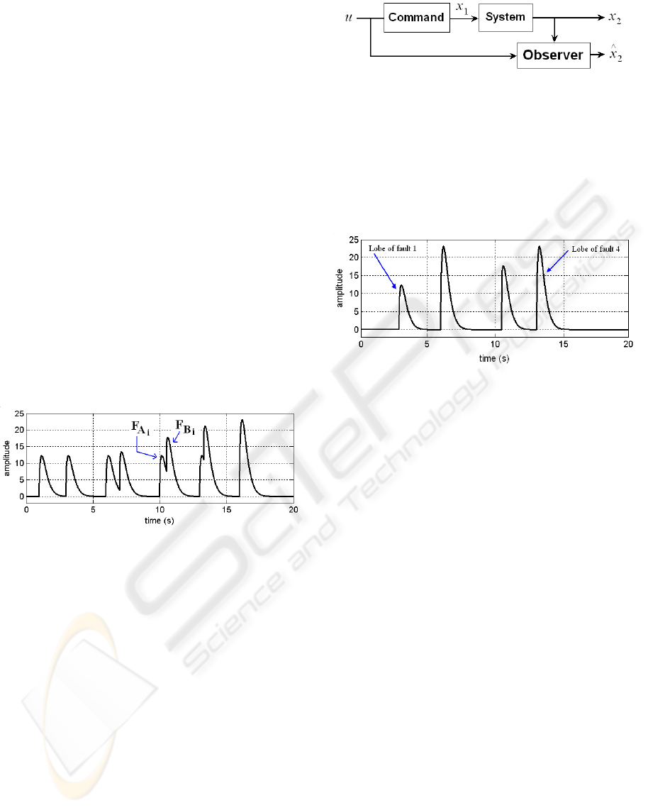
The two only currently available information via the
observers are the representative signal shape of the
fault (residue signal indicating fault) and the measur-
able value of its amplitude. It is possible to detect
with the same residue signal several faults, occurring
at different instants, therefore successively, or at the
same instant (figure 1). However, if we have not ad-
equate tools to detect and to distinguish the various
faults (between F
A
i
and F
B
i
, see figure 1), it is nec-
essary to describe the fault correctly. In that goal, it is
proposed a characterization of fault, which will make
it possible to evaluate its amplitude and its time loca-
tion, and to check its influence on the preceding fault
and/or the following one. This characterization will
also make it possible to conclude on the presence of
one or several faults in the signal, to determine the
local amplitude in the one fault case or total ampli-
tude in a several faults case, and by consequence to
proceed to a correct compensation according to the
fault event instants and fault amplitudes. This is sig-
nificant especially when it is about real time compen-
sation where the dynamic system must be corrected
immediately.
Figure 1: System with parameter observer.
3 OBSERVER BEHAVIOR AND
RESIDUE SIGNAL
The behavior of linear or nonlinear observer with
respect to the faults works according to the following
principle : when a fault occurs on one or some of the
system parameters, given that each parameter have
its own observer, the corresponding observer can
detect the fault and the residue signal changes value
from zero (or close to zero) to a non-zero value, then
it takes a zero value again (or close to zero) after a
considerable short duration.
The figure (2) formalizes an example of an
observing system (Kuo and Golnaraghi, 2003),
(Rosenwasser and Lampe, 2000), where x
1
and
x
2
are state variables and where x
1
is the speed
Figure 2: System with parameter observer.
to observe. The observer is designed to follow
x
1
by knowing the signals x
2
and u. The output
signal of the system is x
2
, and the observer signal
is represented by ˆx
2
which is called the residue signal.
Figure 3: Residue signal : one parameter observation.
With the system as indicated on figure (2) in
presence of faults, one can obtain the simulation
residue signal which is given on figure (3) where four
simulated faults are detected at instants 5, 10, 12 and
16.
The importance here is not to give the transfer
function of the system and doing development to
found characteristic equation of ˆx
2
, but to explicit the
residue signal in order to extract pattern characteris-
tics of some importance. Thus, fault characterization
is concerned by the study of this residue signal and
precisely the Fault Lobe which represents the residue
signal variation from its initial zero or close to zero
value to next zero or close to zero value as shown on
figure (3). However, as it will be seen in section 5,
when faults occur at very close instants, one cannot
distinguish the lobes and will see all them in the same
one lobe. Thus, in a general way, one cannot know
if a lobe corresponds well to only one fault or several
ones.
Because the residue signal can be analyzed and
then some compensator can in such a way compen-
sate the parameter which underwent this fault, this
compensation is reliable only if the characteristics of
the fault are known such as the amplitude (or gain)
and the nature (lobe representing only one fault or
several faults).
ICINCO 2006 - SIGNAL PROCESSING, SYSTEMS MODELING AND CONTROL
128

Suppose that θ is the parameter to be controlled
so that θ
0
is the nominal value (normal functioning of
the system). Let θ
1
the current parameter value. The
error can be defined by :
ε = |θ
1
− θ
0
| (1)
If during control the process, the parameter θ
undergoes a first fault, its observer can detect it and
the compensator will be able thereafter to compensate
the parameter while bringing back ǫ to zero.
Figure 4: Residue signal showing faults occurring at closer
(a) and very closer (b) instants.
The delay between the instant detection of fault
and the instant of the end of compensation, so during
compensation, there can occur n other faults with,
possibly, various amplitudes, sometimes on the same
parameter. If these faults occur at very close instants
(figure 4b), the residue signal will not shows clearly
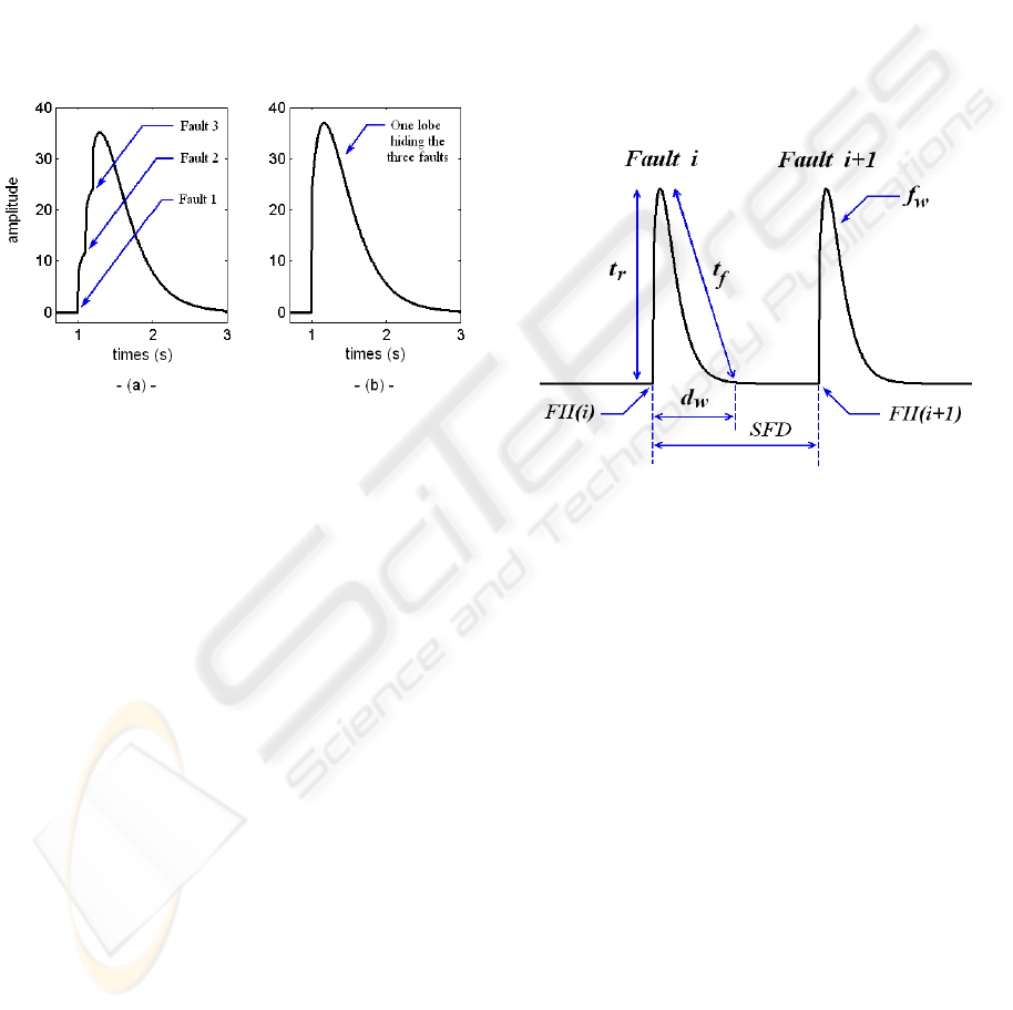
the lobes related to each fault (figure 4a). If the faults
instants are even closer, the residue signal will give a
single lobe hiding thus all the faults lobes. In other
words, these faults are not correctly detectable, the
compensation command signal which is in progress
will not be correct too.
In the next section, it will be highlighted the char-
acterization of a fault, to be an assistance tool to the
faults detection, where all situations of faults occur-
rence and types of detection will be discussed.
4 FAULT CHARACTERIZATION
A system parameter can undergo one or several faults
spread out in time. We have shown in section 3 that
if the faults occur at the same instant or very closer
instants, they can be assimilating to only one fault but
with amplitude more significant than that of each fault
separately (figure 4b). If the faults occur successively,
therefore at different instants, a robust and precise ob-
server must be able to detect them clearly, to distin-
guish them and to have a sufficient resolution of de-
tection, i.e. to detect two clear successive faults over
the one smallest possible duration of incidence, noted
F ID (see Definition 3).
4.1 Definitions
One defines the new following useful terms. Suppose
that i is the fault recurrence number and n is the
number of faults.
Figure 5: Fault characterization in observer residue signal.
The figure (5) shows two well distinguished suc-
cessive faults (i) and (i + 1) at different instants, oc-
curring on a system parameter in fault, where all no-
tations are described in the definitions below.
Definition 1 The instant when the residue, previ-
ously equal to zero or close to zero, starts to change
its value to reach an amplitude different from zero is
defined as F II (Fault Incidence Instant). Therefore
F II(i) is the fault incidence instant of fault i, and
F II(i + 1) is the fault incidence instant of following
fault i + 1 (figure 5).
Definition 2 The duration running out between two
successive faults i and i + 1 (figure 5), is noted SF D
(Successive Fault Duration) and defined by :
SF D = F II (i + 1) − F II (i) (2)
Definition 3 The duration running out between the
instant F II(i) of fault i and the instant when the
residue (corresponding to fault i) takes the value zero
FAULT CHARACTERIZATION FOR MULTI-FAULT OBSERVER-BASED DETECTION IN TIME VARYING
SYSTEMS
129

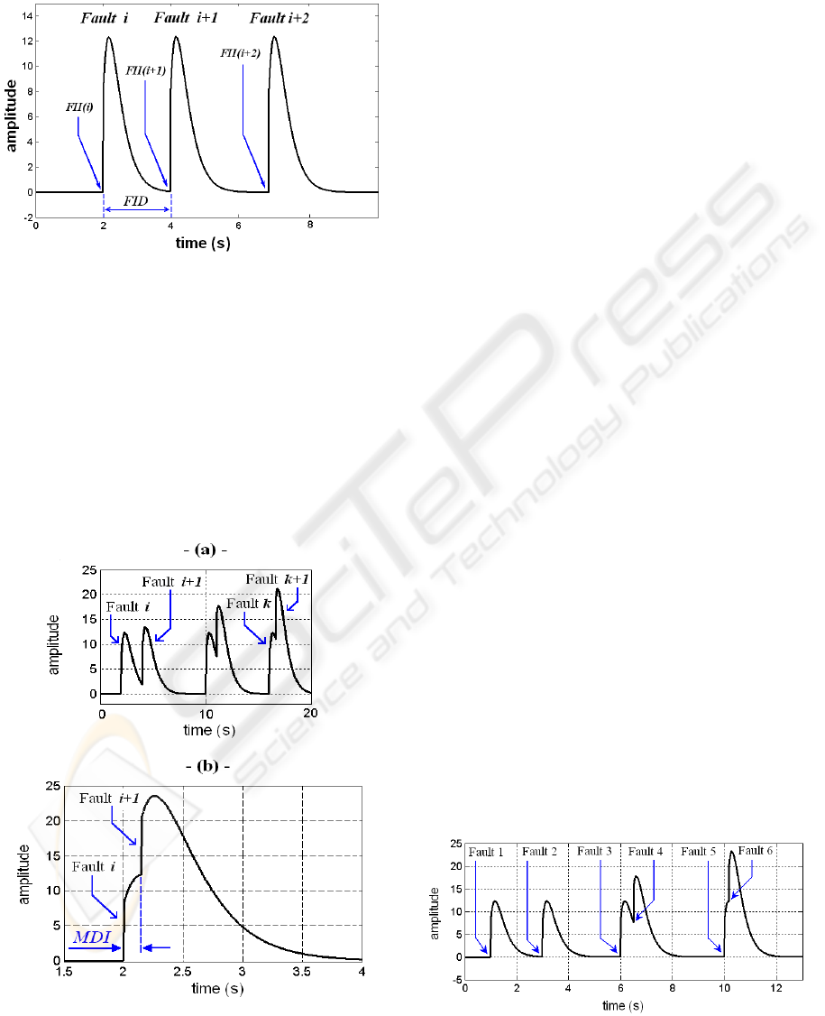
or close to zero is defined as F ID (Fault Incidence
Duration) (figure 6).
Figure 6: Fault Incidence Duration (FID).
Definition 4 The duration between the fault inci-
dence instant F II(i) and the instant when the residue
signal reaches the first maximum value of its ampli-
tude (corresponding to fault i) is noted t
r
(figure 5).
The duration between the instant when the residue
signal has the maximum value of its amplitude and
the instant when it reaches the zero value or close to
zero is noted t
f
(figure 5).
Figure 7: a) Two successive faults. b) Minimum Duration
Incidence (MDI).
If the residue signal contains two faults i and i +
1, one can suppose that at the time when the fault i
took place, that is to say during the variation of the
residue corresponding to this fault, another fault i + 1
intervenes (figure 7a). This assumption leads us to
definition 5.
Definition 5 The duration between the instant
F II(i) and the moment when finishes the raising
time t
r
of fault i, which also corresponds to the be-
ginning of the raising time t
r
of the following fault
i + 1, is defined as MDI (Minimum Duration of In-
cidence) (figure 7b).
Definition 6 The wrap of fault which covers the du-
ration (t
r
+ t
f
) is called fault wrap and noted f
w
(fig-
ure 5).
Definition 7 The duration between the instant
F II(i) and the moment when this residue come back
to zero or close to zero is named a wrap duration and
noted d
w
(figure 5). It is defined by :
d
w
= t
r
+ t
f
(3)
Remark : The term d
w
corresponds to fault com-
plete wrap and will be used in the case of one fault
presence in residue signal. The term F ID corre-
sponds to definitely detected fault and will be used
in the case of multi-fault presence in residue signal.
5 TYPES OF DETECTION
Consider the observer residue signal obtained by sim-
ulation and plotted in figure (8). Six faults are sim-
ulated at instants 1, 3, 6, 6.5, 10 and 10.18 zoomed.
The first two ones are zoomed in figure (9), the two
second ones in figure (10) and the two last ones in
figure (11). Notice that the simulated amplitudes of
all faults are equal.
Figure 8: Multi-faults residue signal.
ICINCO 2006 - SIGNAL PROCESSING, SYSTEMS MODELING AND CONTROL
130

One can notice that the simulation of the figure (8)
shows well the impact of the event of a fault i + 1 for
the length of time d
w
(see figure 5) of the preceding
fault i. Here, the fault-4 intervening during fault-3
lobe took a more significant amplitude than envisaged
(value 17.5 instead of 12), even thing for the fault-6
intervening during the fault-5 lobe. But the fault-2
taking place apart from the fault-1 lobe has a correct
amplitude.
While Basing on the diagram of the figure (8) rep-
resenting the observer signal, three types of detection
can be distinguished and which are complete, partial
and skewed detection.
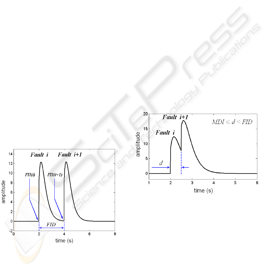
5.1 Complete Detection
If no fault occurs for the length of duration d
w
of fault
i (figure 5), the fault will be clearly and properly de-
tected. This means that the SF D is equal to F ID.
Therefore, to have a clear fault without overlapping
with the next fault i +1 (figures 5 and 9), and in order
to obtain the real values of different faults amplitudes,
the following condition (4) must be satisfied :
SF D
cd
≥ F ID (4)
If the condition (4) is checked, the detection will be
complete (figures 5 and 9) and the compensation will
be able to take place knowing that the fault detection
was correct.
Figure 9: Limit Complete Detection of a fault.
The figure (9) shows the limit of complete detection
which corresponds to equation (5) :
SF D
lcd
= F ID (5)
5.2 Partial Detection
The partial fault detection corresponds to a new fault
detection during the failing time t
f
of the earlier fault
(figure 10). Thus, the detection of a next fault i+1 for
the length of duration d corresponding to the duration
between the beginning of the time t
f
of fault i and the
occurrence of the fault i + 1 during same time t
f
is
considered as partial detection. The duration d can be
defined then by the equation (6) :
MDI ≤ d < F ID (6)
where MDI is minimum duration of incidence
(see Definition 5).
Although the observer has an enough fast response
time to detect the fault, the time t
f
remains rather long
compared to the raising time t
r
(see figure 5). This
means that if other faults occur in the duration d
w
,
they will be partially represented in the residue. The
amplitudes of faults pile up to give to the amplitude
of last fault a different value from what it was nor-
mally to be. This value is not inevitably the sum of
the amplitudes of all faults, but it is more significant
and is not representative. Thus, if the compensation
takes place will not be correct taking into account the
fluctuations in the parameter enduring these faults.
Figure 10: Partial detection of a fault.
5.3 Skewed Detection
Skewed detection (figure 11) corresponds to a new
fault detection (fault i + 1) during or at the end of
the raising time t
r
of the earlier fault (fault i).
6 PROPERTIES
Knowing that every fault has its own wrap, and if sev-
eral faults occur with the condition (7)
FAULT CHARACTERIZATION FOR MULTI-FAULT OBSERVER-BASED DETECTION IN TIME VARYING
SYSTEMS
131

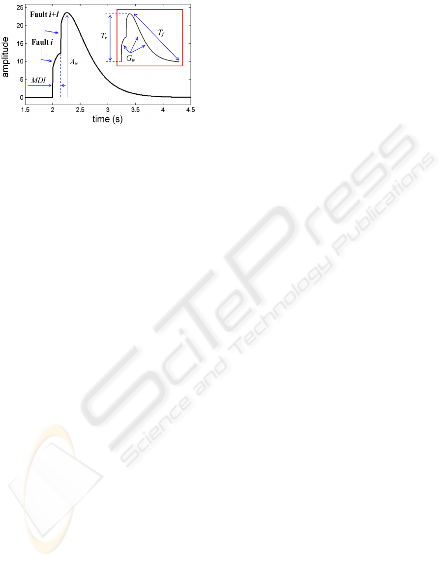
Figure 11: Skewed detection of a fault.
SF D < M DI (7)
all the wraps of faults are reduced to one global
wrap G
w
which is covering the all wraps of the faults
as shown on figure (4b). That gives the impression
thus to detect only one fault with one wrap. The
global wrap, expressed by equations (8) and (9), is
defined by G
w
which is expressed of local wrap func-
tion F
w
i
of each fault i corresponding to its duration
t
r
:
G
w
= F
w
1
+ F
w
2
+ · · · + F
w
n
=
n
X
i=1
F
wi
(8)
F
w
1
∆
= (f
w
)
1
t
r
F
w
1
∆
= (f
w
)
1
t
r
.
.
.
F
w
n
∆
= (f
w
)
n
t
r
(9)
where n is the number of faults and F
w
i
the wrap
of fault i for duration t
r
(i = 1 · · · n),
Really, for n faults, the global raising time T
r
cor-
responds to the pile up of the local times t
r
and the
global failing time T
f
corresponds to the pile up of
the local times t
f
, of all faults which are dissimulated
under the global fault G
w
. So, T
r
and T
f
are non-
linear functions which can be expressed by equations
(10) and (11).
T
r
=
n
X
i=1
α
i
t
r
i
, i = 1 · · · n (10)
T
f
=
n
X
i=1
β
i
t
f
i
, i = 1 · · · n (11)
where α
i
and β
i
are coefficients, t
r
i
the raising
time of fault i and t
f
i
the failing time of fault i.
In normal functioning conditions of observer, the
residue signal, corresponding to system parameter
having undergone these various faults in skewed de-
tection case, will have an end value of amplitude A
(figure 11) which is neither that of the first fault nor
that of the last one. It does not represent also the sum
of the all amplitudes. Or an online compensator inter-
vening during MDI consider only the first fault with
its own amplitude, which is incorrect. The total lobe,
result of the twinning of the all faults lobes, have the
wrap amplitude A
w
which can be written in a nonlin-
ear function expressed by (12).
A
w
=
n
X
i=1
c
i
A
i
(12)
where A
i
is amplitude of fault i, and c
i
its coeffi-
cient.
7 OBSERVER RESOLUTION IN
MULTI-FAULT DETECTION
The encountered problems in partial and skewed de-
tections types has conduce us to consider the M DI
as determining and crucial element for fault detec-
tion resolution. So, one of the consequences of the
fault characterization is the resolution which an ob-
server must take into account to have the best resolv-
ing power between two successive faults. This resolv-
ing power will characterize the observer precision or
resolution to detect two successive completely fault
and without overlapping. So to differentiate between
the precision from the various observers, it is enough
to determine the M DI of each one then to compare
them to conclude which is smallest. Thus, a better
observer would be that which detects all the faults
with their real amplitude some is duration SF D (see
Definition 2), and the best observer resolution would
be that for which the maximum of faults are properly
(completely) detected during the time MDI.
8 CONCLUSION
A system parameter fault represented in a residue sig-
nal by a lobe is characterized in order to determine
its behavior which enable us to treat it correctly and
effectively. The important characteristics of the fault
were largely detailed and new definitions were estab-
lished and which will allow to proceed to a correct
future compensation.
It was highlighted the impact of the occurrence of
several successive faults, at very close instants or at
different instants, on the amplitude of residue signal.
It was given conditions to respect for detecting cor-
rectly one or more faults. It was proven the influence
ICINCO 2006 - SIGNAL PROCESSING, SYSTEMS MODELING AND CONTROL
132

of the detecting response time on fault detection and
compensation.
Two properties are deduced, first the global ampli-
tude of faults occurring at very close instants repre-
sented by the residue amplitude can be represented by
a nonlinear function with coefficients which remains
to be determined, and secondly the resolution to de-
tect two successive completely faults without overlap-
ping. These two properties can be interesting for the
fault compensation.
To carry out a correct detection of all possible
faults, it is necessary that the observer would be pre-
cise and able to distinguish the various faults, some is
instant of incidence, with a good resolution of detec-
tion. In other words, the observer must have a good
resolving power.
REFERENCES
Isermann, R. (1995). Model base fault detection and diag-
nosis methods. Proceedings of the American Control
Conference, 3:1605–1609.
Kuo, B. C. and Golnaraghi, F. (2003). Automatic control
systems. Eds John Wiley and Sons, New York.
Lee, I. S., Kim, J. T., Lee, J. W., Lee, D. Y., and Kim, K. Y.
(2001). Inversion based fault detection and isolation.
Proceedings of the 40th IEEE Conference on Decision
and Control, 2:1005–1010.
Lee, I. S., Kim, J. T., Lee, J. W., Lee, D. Y., and Kim,
K. Y. (2003). Model-based fault detection and isola-
tion method using art2 neural network. International
Journal of Intelligent Systems, 18:1087–1100.
R. Hadj Mokhneche, H. M. and Vigneron, V. (2005). Hy-
brid algorithms for the parameter estimate using fault
detection, and reaching capacities. The 2nd Interna-
tional Conference on Informatics in Control, Automa-
tion and Robotics ICINCO, Barcelona, Spain, 4:289–
293.
Rosenwasser, E. N. and Lampe, B. P. (2000). Computer
controlled systems: Analysis and design with process-
orientated models. Eds. Springer, New York.
Shen, L. C. and Hsu, P. L. (1998). Robust design of fault
isolation observers. Automatica, 34:1421–1429.
V. Venkatasubramanian, R. Rengaswamy, K. Y. and Kavuri,
S. N. (2003a). A review of process fault detection and
diagnosis. part i: Quantitative model-based methods.
Computers and Chemical Engineering, 27:293–311.
V. Venkatasubramanian, R. R. and Kavuri, S. N. (2003b). A
review of process fault detection and diagnosis. part ii:
Qualitative models and search strategies. Computers
and Chemical Engineering, 27:313–326.
V. Venkatasubramanian, R. Rengaswamy, S. N. K. and Yin,
K. (2003). A review of process fault detection and di-
agnosis. part iii: Process history based methods. Com-
puters and Chemical Engineering, 27:327–346.
Vemuri, A. T. and Polycarpou, M. M. (1997). Robust non-
linear fault diagnosis in input-output systems. In-
ternational Journal of Control, Taylor and Francis,
68:343–360.
Xiong, Y. and Saif, M. (2000). International journal of
robust and nonlinear control. Automatica, 10:1175–
1192.
FAULT CHARACTERIZATION FOR MULTI-FAULT OBSERVER-BASED DETECTION IN TIME VARYING
SYSTEMS
133