MULTIPLE MOBILE ROBOTS MOTION-PLANNING: AN

APPROACH WITH SPACE-TIME MCA

Fabio M. Marchese

Dipartimento di Informatica, Sistemistica e Comunicazione

Universit

a degli Studi di Milano - Bicocca

Via Bicocca degli Arcimboldi 8, I-20126, Milan (Italy)

Keywords:

Mobile Robots, Motion Planning, Cellular Automata, Trajectories Generation.

Abstract:

In this paper is described a fast Path-Planner for Multi-robot composed by mobile robots having generic

shapes and sizes (user deﬁned) and different kinematics. We have developed an algorithm that computes the

shortest collision-free path for each robot, from the starting pose to the goal pose, while considering their

real shapes, avoiding the collisions with the static obstacles and the other robots. It is based on a directional

(anisotropic) propagation of attracting potential values in a 4D Space-Time, using a Multilayered Cellular

Automata (MCA) architecture. This algorithm makes a search for all the optimal collision-free trajectories

following the minimum valley of a potential hypersurface embedded in a 5D space.

1 INTRODUCTION

In this paper we describe a safe path-planning tech-

nique for multiple robots based on Multilayered Cel-

lular Automata (MCA). The aim is to design a Co-

ordinator for multi-robot systems which decides the

motions of a team of robots while interacting with the

environment and reacting as fast as possible to its dy-

namical events. Many authors have proposed differ-

ent solutions during the last twenty-ﬁve years, based,

for example, on a geometrical description of the en-

vironment (e.g. (Lozano-P

erez and Wesley, 1979;

Lozano-P

erez, 1983)). The path-planners working on

these types of models generate very precise optimal

trajectories and can solve really difﬁcult problems,

also taking into account non-holonomic constraints,

but they are very time consuming, too. In our opin-

ion, to face a real dynamical world, a robot must con-

stantly sense the world and re-plan accordingly to the

new acquired information. Other authors have de-

veloped alternative approaches less precise, but more

efﬁcient: the Artiﬁcial Potential Fields Methods. In

the eighties, Khatib (Kathib, 1985) ﬁrst proposed this

method for the real-time collision avoidance problem

of a manipulator in a continuous space. Jahanbin

and Fallside ﬁrst introduced a wave propagation al-

gorithm in the Conﬁguration Space (C-Space) on dis-

crete maps (Distance Transform (Jahanbin and Fall-

side, 1988)). In (Barraquand et al., 1992), the au-

thors used the Numerical Potential Field Technique

on the C-Space to build a generalized Voronoi Dia-

gram. Zelinsky extended the Distance Transform to

the Path Transform (Zelinsky, 1994). Tzionas et al.

in (Tzionas et al., 1997) described an algorithm for

a diamond-shaped holonomic robot in a static envi-

ronment, where they let a CA to build a Voronoi Dia-

gram. In (Warren, 1990) is proposed the coordination

of robots using a discretized 3D C-Space-Time (2D

workspace and time) for robots with the same shape

(only square and circle) and a quite simple kinematics

(translation only). La Valle in (LaValle and Hutchin-

son, 1998) applies the concepts of the Game Theory

and multiobjective optimization to the centralized and

decoupled planning. A solution in the C-Space-Time

is proposed in (Bennewitz et al., 2001), where the au-

thors use a decoupled and prioritized path planning

in which they repeatedly reorder the robots to try to

ﬁnd out a solution. It can be proofed that these ap-

proaches are not complete. In this paper, we have

used CA as a formalism for merging a grid model of

the world (Occupancy Grid) with the C-Space-Time

of multiple robots and Numerical (Artiﬁcial) Poten-

tial Field Methods, with the purpose to give a simple

and fast solution for the path-planning problem for

multiple mobile robots, in particular for robots with

different shapes and kinematics. This method uses a

directional (anisotropic) propagation of distance val-

ues between adjacent automata to build a potential hy-

398

Marchese F. (2006).

MULTIPLE MOBILE ROBOTS MOTION-PLANNING: AN APPROACH WITH SPACE-TIME MCA.

In Proceedings of the Third International Conference on Informatics in Control, Automation and Robotics, pages 398-403

DOI: 10.5220/0001218103980403

 SciTePress

persurface embedded in 5D space. Applying a con-

strained version of the descending gradient on the hy-

persurface, it is possible to ﬁnd out all the admissible,

equivalent and shortest (for a given metric of the dis-

cretized space) trajectories connecting two positions

for each robot C-Space-Time.

2 PROBLEM STATEMENTS

A wide variety of world models can be used to de-

scribe the interaction between an autonomous agent

and its environment. One of the most important is the

Conﬁguration Space (Latombe, 1991; Lozano-P

erez,

1983). The C-Space C of a rigid body is the set of all

its conﬁgurations q (i.e. poses). If the robot can freely

translate and rotate on a 2D surface, the C-Space is a

3D manifold R

× SO(2). It can be modelled using

a 3D Bitmap GC (C-Space Binary Bitmap), a regular

decomposition in cells of the C-Space, represented by

the application GC : C → {0, 1}, where 0s represent

non admissible conﬁgurations. The C-Potential is a

function U(q) deﬁned over the C-Space that ”drives”

the robot through the sequence of conﬁguration points

to reach the goal pose (Barraquand et al., 1992). Let

us introduce some other assumptions: 1) space topol-

ogy is ﬁnite and planar; 2) the robot has a lower bound

on the steering radius (non-holonomic vehicle). The

latter assumption introduces important restrictions on

the types of trajectories to be found.

Cellular Automata are automata distributed on the

cells of a Cellular Space Z

(a regular lattice) with

transition functions invariant under translation (Goles

and Martinez, 1990): f

(·) = f (·), ∀c ∈ Z

, f (·) :

→ Q, where c is the coordinate vector identi-

fying a cell, Q is the set of states of an automaton and

is the set of arcs outgoing from a cell to the neigh-

bors. The mapping between the Robot Path-Planning

Figure 1: MultiLayers Architecture.

Problem and CA is quite simple: every cell of the

C-Space Bitmap GC is an automaton of a CA. The

state of every cell contributes to build the C-Potential

U(q) through a diffusion mechanism between neigh-

bors. The trajectories are found following the mini-

mum valley of the surface U(q). In this work, we use

a simple extension of the CA model: we associate a

vector of attributes (state vector) to every cell. Each

state vector depends on the state vectors of the cells

in the neighborhood. There is a second interpretation:

this is a Multilayered Cellular Automaton (Bandini

and Mauri, 1999), where each layer corresponds to

a subset of the state vector components. Each sub-

set is evaluated in a single layer and depends on the

same attribute of the neighbor cells in the same layer

and depends also on the states of the corresponding

cell and its neighbors in other layers. In the follow-

ing sections, we describe each layer and the transition

function implemented in its cells.

3 MULTILAYERED

ARCHITECTURE

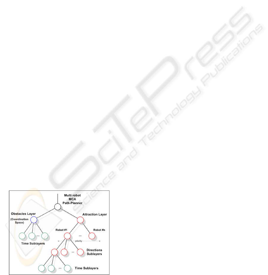
In Fig. 1 is shown the layers structure and their de-

pendencies. There are two main layers: Obstacles

Layer and the Attraction Layer. Each layer is sub-

divided in more sublayers: the Obstacles L. has 3 di-

mensions (2 for the workspace (X, Y ) and 1 more for

the time), while the Attraction L. has up to 5 dimen-

sions (1 for the robots, 2 for the robots workspaces +

1 for their orientations (X, Y, Θ) and 1 for the time).

In the following subsections, we will brieﬂy describe

each layer and their roles. The Obstacles L. concep-

tually depends on the outside environment. Its sub-

layers have to react to the ”external” changes: the

changes of the environment, i.e. the movements of

the obstacles in a dynamical world. Through a sen-

sorial system (not described here), these changes are

detected and the information is stored in Obstacles L.

permitting the planner to replan as needed.

3.1 The Obstacles Layer

The main role of the Obstacles Layer is to create a re-

pulsive force in the obstacles to keep the robots away

from them. In the present work, only static obstacles

are considered (e.g. walls). For the single robot, the

other robots are seen as moving obstacles, with un-

known and unpredictable trajectories. We are consid-

ering a centralized planner/coordinator, that can de-

cide (and, of course, it knows) the trajectories of all

the supervised robots. Thanks to this knowledge, the

planner considers the silhouette of the robot as an ob-

stacle for the other robots. In this work, we introduce

a discretized version of the C-Space-Time as in (War-

ren, 1990). With the introduction of the Time axis,

MULTIPLE MOBILE ROBOTS MOTION-PLANNING: AN APPROACH WITH SPACE-TIME MCA

399

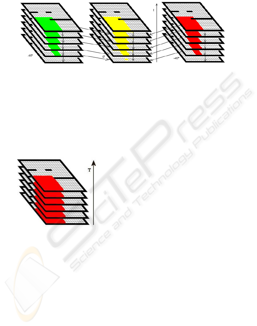
Figure 2: Dependencies between Attractive Layers at different orientations.

the robots moving in the environment become ”static”

obstacles in the Space-Time 4D space, having differ-

ent poses in each time slice. We can still call them as

C-Obstacles, remembering that they are extended in

the time dimension. In our case, we have a 3D Space-

Time: R

×R, where R

is the planar workspace. The

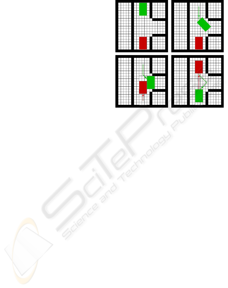
overall ”static” space-time obstacle, representing one

robot, is the composition of all the robot silhouettes

in each time slice (Fig. 3). The time step (slice) is the

Figure 3: Discretized C-Space-Time and C-Obstacles.

time needed by a robot to move to an adjacent cell, if

we consider all the robots moving at the same speed

(the robots motions are synchronized). This layer is

also called Coordination Layer (Space) because the

motion of all the robots are coordinated in this layer

(see 3.3).

3.2 The Attractive Layer

The Attractive Layer is the core of the algorithm. It

computes the shortest collision-free path for a single

robot, from the starting pose to the goal pose, while

considering its real occupation (shape and size = sil-

houette). To pass from one cell to an other one, the

robot can follow different paths, combining different

atomic moves, such as strict forward move, diagonal

move, rotation, and so on. Each move has its own cost

(always positive); the entire set of admissible move-

ments deﬁne the robot kinematics. The planner is able

to handle at the same time different type of robots,

with different shapes, sizes and kinematics (e.g. car-

like kinematics, omnidirectional, etc.), providing for

each one the proper trajectory. In this work, the moves

are space-temporal, i.e. every time the robot moves

in the space, it also moves in the time. Even when

the robot stands in the same place, it moves (verti-

cally) in the space-time (also this particular move has

its own cost). The moves costs are used to build in-

crementally a potential surface starting from the goal

cell, placed at a high time slice (the desired time of

arrival), and expanding it in all the free space-time. In

our case, it is a hypersurface embedded in a 4D space:

× SO(1) × R, where R

is the workspace, en-

larged with the robot orientation dimension (SO(1))

and the time. The goal cell receives the ﬁrst value

(a seed), from which a potential bowl is built adding

the cost of the movement that would bring the robot

from a surrounding cell to it. The calculus is per-

formed by the automata in the space-time cell, which

computes the potential value depending on the poten-

tial values of the surrounding space-time cells. Iter-

ating this process for all the free cells, the potential

surface is built leaving the goal cell with the mini-

mum potential. The potential value has a particular

mean: it is the total (minimal) cost needed to reach

the goal from the current cell. Because the costs are

positive, no other minimum is generated, thus avoid-

ing the well-known problem of the ”local minima”.

The entire trajectory is computed just following the

direction of the negated gradient of the surface from

the starting point. The path results to be at the mini-

mum valleys of the surface. Every robots have differ-

ent goals and kinematics, hence a potential bowl for

each one has to be generated separately. The potential

bowl is built only in the free space, avoiding to enter

in the C-Obstacles areas. Therefore, the robot Attrac-

tive Layer depends on the Obstacles Layer. The last

one embeds the Time, thus the potential bowl varies

with the time, generating different potential surfaces

ICINCO 2006 - ROBOTICS AND AUTOMATION

400

at different starting time and, consequently, different

trajectories. In Fig. 2 is shown the dependencies be-

tween Layers and Sublayers of the overall Attractive

Layer. Each sublayer, at a given robot orientation,

depends on the adjacent sublayers at different orien-

tations (aside in the ﬁgure), and depends also on the

below temporal sublayer.

3.3 The Planning Algorithm

Entailing the layer structure previously introduced, is

now possible to describe the algorithm to compute the

robots trajectories. The ﬁrst step is to establish the

robots priorities. Up to now, no heuristic has been

found and the assignment is casual. The following

step is to initialize the Obstacles Layer with the ob-

stacle distribution known from the Occupancy Map

of the workspace. Each temporal sublayer is set to the

Occupancy Map (full if the cell has an obstacle inside,

empty otherwise). Then, the algorithm computes the

Attractive Layer of the robot with the highest prior-

ity level based on the Obstacles Layer. Setting the

minimum potential value to the goal cell, it makes the

potential bowl growing while surrounding the obsta-

cles. Knowing the potential surface, it extracts the

shortest path, following the negated gradient from the

starting cell. For each passing points, then it adds the

robot silhouettes, properly oriented, in each tempo-

ral sublayer of the Obstacles Layer. In this way, the

ﬁrst robot becomes a space-time ”obstacle” for the

successive robots, with lower priorities. The Obsta-

cles Layer has a central role in this phase, because it

ensures that the robots avoid each other and the tra-

jectories do not intersect each other, even taking into

account their real extensions. For this reason, in this

context it is also called Coordination Space. The next

phase is to repeat the procedure for the second robot,

starting to build its Attractive Layer on the base of the

modiﬁed Obstacles Layer, and then adding to it all its

silhouettes at each time-stamp. The algorithm termi-

nates when it has computed all the robots trajectories.

4 EXPERIMENTAL RESULTS

The priority planning is not complete: there are situ-

ations for which there is a ”natural” simple solution,

but this type of algorithm is not able to ﬁnd it. In

Fig. 4 is shown an example (a similar one in (Ben-

newitz et al., 2001)) of such a type of problems and

a simple solution. Adopting a priority order (e.g. the

green robot moves before the red one) there is no solu-

tion. Because this problem is symmetric, even swap-

ping the priority order (e.g. the red one passes before

the green one) there is still not a solution with a prior-

Figure 4: Counter-example: a situation for which the prior-

ity planning does not ﬁnd a solution.

ity schema. Fortunately, for most of the situations we

do not have this kind of problem and the algorithm

ﬁnds a solution. In the example of Fig. 5, the red

robot has the clear the way to permit the green one

to get out of the room, then it gets back to the orig-

inal position. The following example (Fig. 6) shows

a classical problem where the robots trajectories have

to cross to exchange their positions in the four cor-

ners. In the middle of the environment there is a con-

ﬂict zone where all the robots have to pass. All the

robots start contemporarily, but the red and yellow

robots have to stop to permit the blue and the green

robots (with higher priority levels) to pass. Then also

the red and yellow ones complete their paths.

5 CONCLUSIONS

In this paper we have proposed a decoupled and pri-

oritized path planning algorithm for coordinating a

Multi-Robot composed by mobile robots using a Mul-

tilayered Cellular Automata. One of the main topics is

that we face contemporarily with mobile robots hav-

ing generic shapes and sizes (user deﬁned) and differ-

ent kinematics. It is based on the Priority Planning ap-

proach in the C-Space-Time where the Time has been

added to the normal C-Space. The Priority Planning

is not complete, but it works very well for most of

the problems, ﬁnding all the collision-free equivalent

paths for each robot. The algorithm is also able to

manage the robots orientations, avoiding to waste a

lot of space during the motion, and permitting to ﬁnd

MULTIPLE MOBILE ROBOTS MOTION-PLANNING: AN APPROACH WITH SPACE-TIME MCA

401

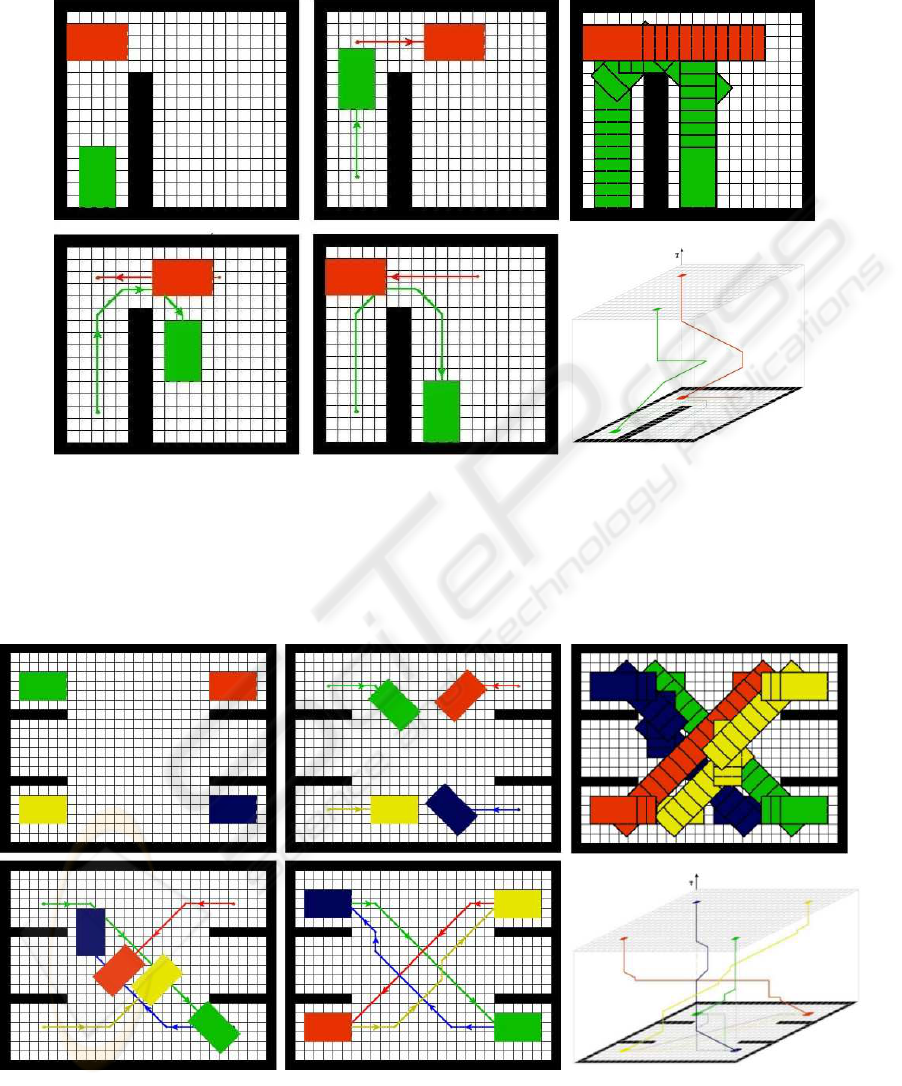
Figure 5: Robot clearing the way: a snapshots sequence (four frames on the left); the overall movements and C-Space-Time

movements.

Figure 6: Crossing robots: a snapshots sequence (four frames on the left); the overall movements and C-Space-Time move-

ments.

ICINCO 2006 - ROBOTICS AND AUTOMATION

402

paths in cluttered workspaces. The trajectories found

are smoothed and respect the kinematics constraints

of each robot.

ACKNOWLEDGEMENTS

The author wish to thank Dott. Marco Dal Negro for

the contributions given with his Graduate Thesis.

REFERENCES

Bandini, S. and Mauri, G. (1999). Multilayered cellular au-

tomata. Theoretical Computer Science, 217:99–113.

Barraquand, J., Langlois, B., and Latombe, J. C. (1992).

Numerical potential ﬁeld techniques for robot path

planning. IEEE Trans. on Systems, Man and Cyber-

netics, 22(2):224–241.

Bennewitz, M., Burgard, W., and Thrun, S. (2001). Op-

timizing schedules for prioritized path planning of

multi-robot systems. In IEEE Int. Conf. on Robotics

and Automation (ICRA), Seoul (Korea).

Goles, E. and Martinez, S. (1990). Neural and Au-

tomata Networks: dynamical behavior and applica-

tions. Kluwer Academic Publishers.

Jahanbin, M. R. and Fallside, F. (1988). Path planning us-

ing a wave simulation technique in the conﬁguration

space. In Artiﬁcial Intelligence in Engineering: Ro-

botics and Processes (J. S. Gero ed.), Southampton.

Computational Mechanics Publications.

Kathib, O. (1985). Real-time obstacle avoidance for ma-

nipulator and mobile robots. In Int. Conf. on Robotics

and Automation.

Latombe, J. C. (1991). Robot Motion Planning. Kluwer

Academic Publishers, Boston, MA.

LaValle, S. M. and Hutchinson, S. A. (1998). Optimal

motion planning for multiple robots having indepen-

dent goals. IEEE Trans. on Robotics and Automation,

14(6):912–925.

Lozano-P

erez, T. (1983). Spatial planning: A conﬁgura-

tion space approach. IEEE Trans. on Computers, C-

32(2):108–120.

Lozano-P

erez, T. and Wesley, M. A. (1979). An algo-

rithm for planning collision-free paths among polyhe-

dral obstacles. Comm. of the ACM, 22(10):560–570.

Tzionas, P. G., Thanailakis, A., and Tsalides, P. G. (1997).

Collision-free path planning for a diamond-shaped ro-

bot using two-dimensional cellular automata. IEEE

Trans. on Robotics and Automation, 13(2):237–250.

Warren, C. (1990). Multiple robot path coordination us-

ing artiﬁcial potential ﬁelds. In Proc. of the IEEE

Int. Conf. on Robotics and Automation (ICRA), pages

500–505.

Zelinsky, A. (1994). Using path transforms to guide the

search for ﬁndpath in 2d. Int. J. of Robotics Research,

13(4):315–325.

MULTIPLE MOBILE ROBOTS MOTION-PLANNING: AN APPROACH WITH SPACE-TIME MCA

403